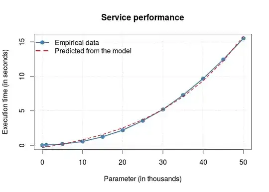
I would like to fit a model and the smallest predicted value must be zero. This is what I have done:
xx = c(.001,1,seq(5,50,5))*1e3
yy = c(0.0001,0.0378,0.1778,0.5422,1.2304,2.1918,3.575,5.1964,
       7.2778,9.6814,12.4536,15.5136)
dat = data.frame(x=xx,y=yy)

# see: http://stats.stackexchange.com/a/160575/86260
c.0 = min(yy) * .5
model.0 = lm(log(y - c.0) ~ x, data = dat)
start = list(a=coef(model.0)[1], b=coef(model.0)[2], c=c.0)
mod = nls(y ~ a * exp(b*x) + c, data = dat, start = start)

zero = predict(mod, list(x = 0))
print(paste('zero:', zero))

# Plot empirical vs. predict
plot(dat$x/1e3,dat$y, xlab = 'Parameter (in thousands)',
     ylab = 'Execution time (in seconds)', main = 'Service performance',
     col = 'steelblue', type = 'o', pch = 19, lwd = 3)
lines(dat$x/1e3, predict(mod, list(x = dat$x)), col = 'red',
      lty = 2, lwd = 2)
grid()
legend('topleft', legend = c('Empirical data',
       'Predicted from the model'), col = c('steelblue', 'red'),
       lwd = 3, lty = c(1,2), pch = c(19,32), bty = 'n')
Which will outputs:
[1] "zero: -0.326332998543469"
As it can be seen, the predicted value for the parameter .001 must be zero (or as close as it is possible of).
How could I fit a model with such a constraints?
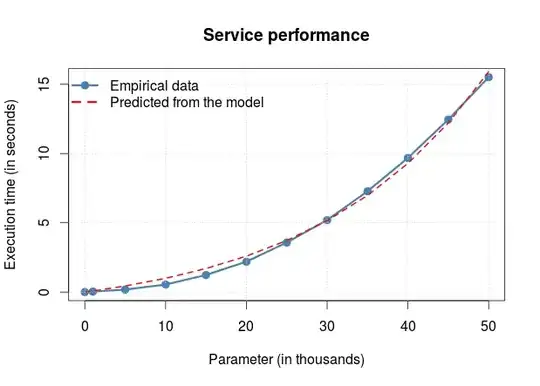
EDIT: an algebraic manipulation can be used to overcome this issue. (thank you @whuber)
The code now become:
xx = c(.001,1,seq(5,50,5))*1e3
yy = c(0.0001,0.0378,0.1778,0.5422,1.2304,2.1918,3.575,5.1964,
       7.2778,9.6814,12.4536,15.5136)
dat = data.frame(x=xx,y=yy)

# see: http://stats.stackexchange.com/a/160575/86260
a.0 = 0
model.0 = lm(log(y - a.0) ~ x, data = dat)
start = list(a=coef(model.0)[1], b=coef(model.0)[2])
mod = nls(y ~ a * exp(b*x) - a, data = dat, start = start)

zero = predict(mod, list(x = 0))
print(paste('zero:', zero))

# Plot empirical vs. predict
plot(dat$x/1e3,dat$y, xlab = 'Parameter (in thousands)',
     ylab = 'Execution time (in seconds)', main = 'Service performance',
     col = 'steelblue', type = 'o', pch = 19, lwd = 3)
lines(dat$x/1e3, predict(mod, list(x = dat$x)), col = 'red',
      lty = 2, lwd = 2)
grid()
legend('topleft', legend = c('Empirical data',
       'Predicted from the model'), col = c('steelblue', 'red'),
       lwd = 3, lty = c(1,2), pch = c(19,32), bty = 'n')
Which will outputs:
[1] "zero: 0"

