Degenerate Model Output for `lmer` Coefficients: What's the Problem and a Possible Fix

Question

This is probably an embarrassingly easy question, but where else can I turn to...

I'm trying to put together examples of regression with mixed effects using lmer {lme4}, so that I can present [R] code that automatically downloads toy datasets in Google Drive and run every instance in this blockbuster post.

And starting with the first case (i.e. V1 ~ (1|V2) + V3, where V3 is a continuous variable acting as a fixed effect, and V2 is Subjects, both trying to account for V1, a continuous DV), I was expecting to retrieve different intercepts for each one of the Subjects and a single slope for all of them. Yet, this was not the case consistently.

I don't want to bore you with the origin or meaning of the datasets below, because I'm sure most of you get the idea without much explaining. So let me show you what I get... If you're so inclined you can just copy and paste in [R]... it should work if you have {lme4} in your Environment:

Expected Output:

politeness <- read.csv("http://www.bodowinter.com/tutorial/politeness_data.csv")
head(politeness)

  subject   gender scenario  attitude frequency
1      F1      F        1      pol     213.3
2      F1      F        1      inf     204.5
3      F1      F        2      pol     285.1
4      F1      F        2      inf     259.7    


library(lme4)

fit <- lmer(frequency ~ (1|subject) + attitude, data = politeness)

coefficients(fit)
            $subject
               (Intercept) attitudepol
            F1    241.1352   -19.37584
            F2    266.8920   -19.37584
            F3    259.5540   -19.37584
            M3    179.0262   -19.37584
            M4    155.6906   -19.37584
            M7    113.2306   -19.37584

Surprising Output:

library(gsheet)
recall <- read.csv(text = 
    gsheet2text('https://drive.google.com/open?id=1iVDJ_g3MjhxLhyyLHGd4PhYhsYW7Ob0JmaJP8MarWXU',
              format ='csv'))
head(recall)

 Subject Time Emtl_Value Recall_Rate Caffeine_Intake
1     Jim    0   Negative          54              95
2     Jim    0    Neutral          56              86
3     Jim    0   Positive          90             180
4     Jim    1   Negative          26             200

fit <- lmer(Recall_Rate ~ (1|Subject) + Caffeine_Intake, data = recall)

coefficients(fit)
        $Subject
               (Intercept) Caffeine_Intake
        Jason     51.51206        0.013369
        Jim       51.51206        0.013369
        Ron       51.51206        0.013369
        Tina      51.51206        0.013369
        Victor    51.51206        0.013369

Here is the output of (summary(fit)):

Linear mixed model fit by REML ['lmerMod']
Formula: Recall_Rate ~ (1 | Subject) + Caffeine_Intake
   Data: recall

REML criterion at convergence: 413.9

Scaled residuals: 
     Min       1Q   Median       3Q      Max 
-1.54125 -0.98422  0.04967  0.81465  1.83317 

Random effects:
 Groups   Name        Variance Std.Dev.
 Subject  (Intercept)   0.0     0.00   
 Residual             601.2    24.52   
Number of obs: 45, groups:  Subject, 5

Fixed effects:
                Estimate Std. Error t value
(Intercept)     51.51206    5.92408   8.695
Caffeine_Intake  0.01337    0.03792   0.353

Correlation of Fixed Effects:
            (Intr)
Caffen_Intk -0.787

Question:

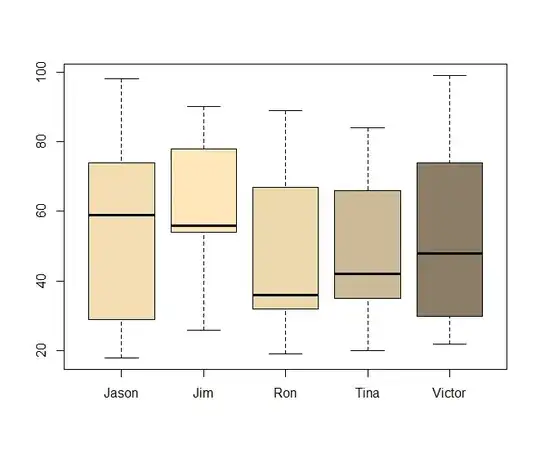
Why are all the Intercepts for the different subjects the same in the second example? The structure of the datasets and the lmer syntax appear very similar... and the boxplots don't seem to support the result:

Thank you in advance!

Answer 1

OK, thanks to @CliffAB tip off, I could track this answer, which addresses the issue head on.

So using the packagae {blme} and reformulating:

require(blme)
fit <- blmer(Recall_Rate ~ (1|Subject) + Caffeine_Intake, data = recall)

coefficients(fit)

$Subject
       (Intercept) Caffeine_Intake
Jason     52.77409     0.007706907
Jim       54.76766     0.007706907
Ron       49.87873     0.007706907
Tina      51.18756     0.007706907
Victor    52.43256     0.007706907

Isn't [R] the best? Plausible... I can see that Ron is showing the worst recall rate, consistent with the boxplot...

But, since we are dealing with a toy data set, I can simply decrease or increase the Recall_Rate for Jim some random percentage, say 20%, and do the same for each one of the subjects (different percentage changes for each individual) so as to make them more distinct from each other. Saved in a separate file, I can now call the following regular lmer function:

recall <- read.csv(text = 
gsheet2text('https://docs.google.com/spreadsheets/d/1FPaU-UoWT95wic1PYiWdukuhKwuLxyDPGeedv64VYvY/edit?usp=sharing',
          format ='csv'))
head(recall)
require(lme4)
fit <- lmer(Recall_Rate ~ (1|Subject) + Caffeine_Intake, data = recall)
coefficients(fit)

And we get different coefficients for each individual:

$Subject
       (Intercept) Caffeine_Intake
Jason     56.06593     -0.01419912
Jim       50.89693     -0.01419912
Ron       42.61979     -0.01419912
Tina      60.98722     -0.01419912
Victor    62.09119     -0.01419912

Evidently this is a luxury only affordable with a toy dataset - real data can't be modified.

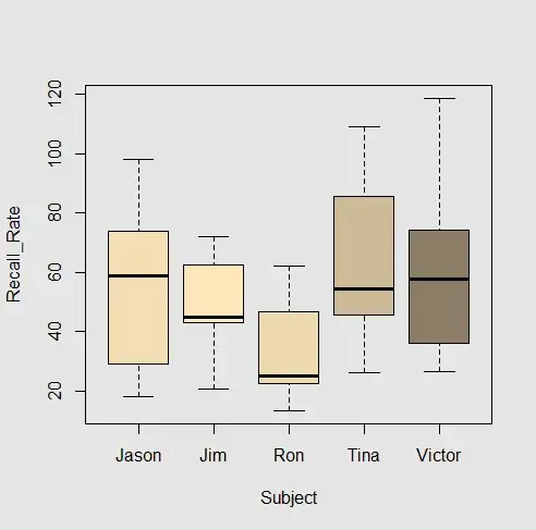
Let's see the boxplot for this new, non-degenerated, dataset:

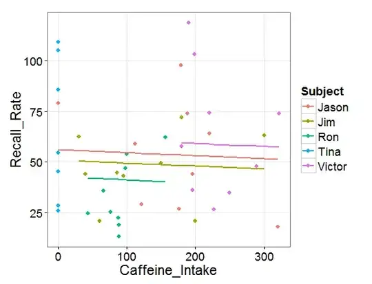
Here is the plot of the different predicted lines color-coded by individual:

All individuals share the same slope, but different intercepts.