Testing the Validity of a Test Statistic (incorrectly)

Question

In this post @Wolfgang shares a few lines of code to test in a simulation the ability of a particular test statistic to perform as expected, measured by the percentage of type I errors. He shows by simulation how the $chi \,square$ test works in the case presented in that original post, despite the small number of "successes" in comparison with the large number of observations.

On a post I wrote to sort of piece together what I've been collecting from many other posts on comparison of proportions, I was trying to come up with a similar type of simulation using the $z$-test. I understand that the $\chi^2$ is mathematically equivalent in this situation, but it was one of these exercises in convincing oneself, and understand the $z \,test$ equations. Further, I wasn't sure the tests were going to be identical in every respect.

So to the question... I road-tested the equation of the $z$ test function, and it did not produce the expected results. The same happened with a similar ad hoc formula in R-Bloggers, which I will use in the rest of the question.

My bet is that my code is flawed (in which case, I'd like to fix it on my prior post), but the values it generates seem plausible; the only odd result being the proportion of type I errors. So I wonder if I could get some help, especially if the results are accurate, and the statistical interpretation is incorrect.

This is the actual problem (more details here if needed):

DATA:

           Medication
Symptoms    Drug A Drug B Totals
  Heartburn     64     92    156
  Normal       114     98    212
  Totals       178    190    368

TEST STATISTIC FUNCTION IN R (from R-Bloggers):

For reference: $ Z = \frac{\frac{x_1}{n_1}-\frac{x_2}{n_2}}{\sqrt{p\,(1-p)(1/n_1+1/n_2)}}$ with $ p = \frac{x_1\,+\,x_2}{n_1\,+\,n_2}$

z.prop = function(x1,x2,n1,n2){
  numerator = (x1/n1) - (x2/n2)
  p.common = (x1+x2) / (n1+n2)
  denominator = sqrt(p.common * (1-p.common) * (1/n1 + 1/n2))
  z.prop.ris = numerator / denominator
  return(z.prop.ris)
}

POPULATION SET UP WITH ONE SINGLE (AVERAGE) TRUE PROPORTION:

set.seed(5)

# Number of samples taken to obtain different proportions IF 
# we set it up so that the proportions are actually equal:

samples <- 100000

# Number of cases for Drug A and Drug B:

n1 <- 178
n2 <- 190

# Proportion of patients with heartburn:
p1 <- 64/n1
p2 <- 92/n2

# We will make up a population where the proportion of heartburn suffers
# is in between p1 and p2:

(c(p <- mean(c(p1, p2)), p1, p2))
[1] 0.4218805 0.3595506 0.4842105

# And we'll take samples of the size of the groups assigned to Drug A 
# and Drug B respectively:

x1 <- rbinom(samples, n1, p)
x2 <- rbinom(samples, n2, p)

# Double - checking that the proportion is kept although the number of
# successes is different:

(c(mean(x1),mean(x2)))
[1] 75.08542 80.15841
(c(prop1 <- mean(x1)/n1, prop2 <- mean(x2)/n2, p))
[1] 0.4218282 0.4218864 0.4218805

SIMULATION:

# Now we run the z-test in what we just did, but we repeat it 100000 times     
# and put the results in vector pval:

pval <- 0
for (i in 1:100000) {
    pval[i] <- pnorm(-abs(z.prop(mean(x1[i]), mean(x2[i]), n1, n2)))
}

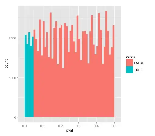
# What is the fraction of pval's below 0.05 (it should be 0.05 since we
# should only reject 0.05 times the true NULL):

mean(pval <= .05)
[1] 0.09887

To my surprise, the result is 0.09887, and changing the set.seed ends up with larger proportions of falsely rejected null hypothesis.

Answer 1

And I want to let you all know that I was absolutely right: my code was flawed! Thanks a million to @Scortchi for walking me through the problem. Since at least two people up-voted the question, here is the answer:

The probability integral function dictates that if $X \sim N(\mu,\sigma^2)$, the random variable $Y = \Phi(X)$ with $\Phi$ corresponding to the error function ($erf$) (who came up with this name?) will be uniformely distributed as $Y \sim U(a,b)$.

Since we know that the $p-values$ range from $(0,1)$, plotting the histogram should illustrate our expectation (overabundant $p<0.05$ values colored in greenish hue):

So we are getting just half of the span we expected: from $[0,0.5]$, as opposed to $[0,1]$. And the problem is in the code treatment of the $z$ values produced by the function z.prop. Since $z$ is a symmetric distribution the part of the code intended to "look up the probability in the table at the end of the book": (pnorm(-abs(z.prop(mean(x1[i]), mean(x2[i]), n1, n2)))) is effectively sending all the $z$ values above $0$ to the negative part of the bell curve, and we end up with double amount of pval < 0.05.

As @Scortchi says in his comments, if you happened to get a $z=1.4$, "you are calculating $Pr(Z<−1.4)$ when you should be calculating $Pr(Z<−1.4)+Pr(Z>1.4)$.

This can be fixed by simply doubling the value of the pvalues. Or perhaps more neatly by changing the SIMULATION part of the code in the OP to:

pval <- 0
for (i in 1:100000) {
     pval[i] <- pnorm(z.prop(mean(x1[i]), mean(x2[i]), n1, n2))
}
> mean(pval <= .025) + mean(pval >= 0.975)
[1] 0.04923