Interpretation of log transformed predictor neatly explains how to interpret a log transformed predictor in OLS. Does the interpretation change if there are 0s in the data and the transformation becomes log(1 + x) instead?
Some authors (e.g. Fox and Weisberg 2011) recommend adding a start (i.e. a positive constant) if a log transformation is necessary to correct skewness and improve symmetry, but the data contains zeros.
Consider a variation of the Ornstein example in CAR (p. 303):
require(car)
data(Ornstein)
boxplot(Ornstein$interlocks, horizontal = T)
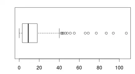
The data is clearly right skewed, and contains 0s.
summary(powerTransform(1 + Ornstein$interlocks))
## bcPower Transformation to Normality
##
##                         Est.Power Std.Err. Wald Lower Bound Wald Upper Bound
## 1 + Ornstein$interlocks    0.1248    0.053           0.0209           0.2287
##
## Likelihood ratio tests about transformation parameters
##                              LRT df      pval
## LR test, lambda = (0)   5.502335  1 0.0189911
## LR test, lambda = (1) 262.431991  1 0.0000000
The powerTransform() function suggests that a log(1 + x) transformation here could be useful.
boxplot(log(1 + Ornstein$interlocks), horizontal = T)
As you can see, symmetry is indeed improved.
Question: If this transformed variable were to be included in an OLS regression as an IV, would the coefficient estimates still have the usual interpretation of log transformed variables?