I have a dataset with multiple samples of batches of observations (e.g. one batch of 20 obs., one batch of 50 obs,, etc.). There is a probability that the batches have contaminated observations, with the number of contaminated observations in each batch following a binomial distribution with a constant probability across batches. However--due to the testing equipment--one only observes whether a batch is contaminated (if there are 1 or latent contaminated samples) or not contaminated. Is there a standard model / R package / formula to calculate the maximum likelihood estimate of the probability?
Asked
Active
Viewed 755 times
2 Answers
6
Let the constant probability of contamination be $p$, which is to be estimated, and let $X$ be a random variable equal to $1$ when contamination is observed, $0$ otherwise. Writing $q=1-p$ for the chance of no contamination in any individual unit, the probability of observing no contamination (that is, $X=0$) in a batch of size $n$ ($n = 1, 2, 3, \ldots$) is $q^n$, whence the chance of observing contamination is
$$\Pr(X=1\,|\, n) = 1 - q^n.$$
In a dataset of independent observations $\mathbf{x} = (x_1, x_2, \ldots)$ of $X$ from batches of size $\mathbf{n} = (n_1, n_2, \ldots)$, the likelihood therefore is
$$L(q; \mathbf{x}, \mathbf{n}) = \prod_{x_i=1} \left(1 - q^{n_i}\right)\prod_{x_j=0} q^{n_j},$$
whence the log likelihood is
$$\Lambda(q) = \sum_{x_i=1} \log\left(1 - q^{n_i}\right) + \sum_{x_j=0} {n_j} \log q.$$
At the extremes $q\to 0$ or $q\to 1$ this continuous function obviously diverges to $-\infty$, implying it has a global maximum somewhere in the interval $(0,1)$ corresponding to a zero of the derivative
$$\frac{d}{d q} \Lambda(q) = -\sum_{x_i=1} \frac{n_i q^{n_i-1}}{1 - q^{n_i}}+ \sum_{x_j=0} \frac{n_j} {q}.$$
Upon multiplying by $q$, the zeros are seen to be the solutions of the equation
$$\sum_{x_i=1} n_i\left( \frac{1}{1 - q^{n_i}}\right) - \sum_{x_i=1}n_i = \sum_{x_i=1} n_i\left( \frac{1}{1 - q^{n_i}}-1\right)= \sum_{x_i=1} \frac{n_i q^{n_i}}{1 - q^{n_i}}= \sum_{x_j=0} n_j.$$
Write, therefore, $N = \sum_{i} n_i$, obtaining
$$\sum_{x_i=1} \frac{n_i}{1 - q^{n_i}} = N.$$
Because for any $k\ge 1$ the function $q\to 1/(1-q^k)$ increases monotonically from $1$ to $\infty$ when $0\lt q \lt 1$, the left hand side increases monotonically from $\sum_{x_i=1}n_i$, which does not exceed $N$. Consequently there is a unique solution $0 \lt \hat q \lt 1$. It can quickly be found using any decent root finder. The estimated probability of contamination is $\hat p = 1 - \hat q$. Confidence intervals, etc., can be found with the usual Maximum Likelihood machinery.
So much information is lost in observing $X$ that these estimates will not be precise. Even with large batches (in the hundreds) and a large number of batches (in the hundreds), when $p$ is small (as one would expect), its estimate $\hat p$ can easily err by a factor of $2$ or greater. Estimates will be particularly poor when few or almost all of the batches exhibit contamination. This prognosis is borne out by the simulation results shown below, which present histograms of the estimates relative to $p$ (that is, the ratios $\hat{p}/p$) and scatterplots of the fraction of contaminated batches (the mean of the $x_i$) against the estimates $\hat p$.
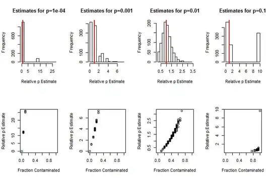
Simulation results for $20$ batches averaging about $40$ units per batch.
Here is the R code that produced this figure. It turns out that minimizing the square of the objective function is a little more accurate and faster than finding its root in $(0,1)$, so optimize was chosen to perform the calculations.
n.batch <- 20                        # Number of batches
set.seed(17)
sizes <- (1+rpois(n.batch, 3)) * 10  # Batch sizes
#
# Simulate data for various values of p and show the distribution of estimates.
#
f <- function(q, x, n) sum((n / (1 - q^n))[x]) - sum(n)
par(mfcol=c(2,4))
for (p in c(1e-4, 1e-3, 1e-2, 1e-1)) {
  p.hat <- replicate(1e3, {
    x <- rbinom(length(sizes), sizes, p) > 0
    solution <- optimize(function(q) f(q, x, sizes)^2,
                         lower=1e-16, upper=1-1e-16, tol=1e-8)
    c(sum(x), 1 - solution$minimum)
  })
  hist(p.hat[2,]/p, main=paste0("Estimates for p=", p), xlab="Relative p Estimate")
  abline(v=1, col="Red", lwd=2)
  plot(p.hat[1,]/n.batch, p.hat[2,]/p, xlim=c(0,1),
       xlab="Fraction Contaminated", ylab="Relative p Estimate")
}
whuber
- 281,159
- 54
- 637
- 1,101
-
Many thanks for that! I was just working on the same problem, but also require the 95% confidence intervals. If phat is 1-optimize(function(q) f(q, x, sizes)^2, lower=1e-16, upper=1-1e-16, tol=1e-8)$minimum, would you know how to calculate the 95% confidence limits on that estimate by any chance? – Tom Wenseleers Jun 28 '16 at 17:38
-
Ha and was also wondering if these likelihood calculations have been published somewhere, and if this problem is perhaps known under a standard name? Just that I would ideally like to give a citation for this in a paper of mine... – Tom Wenseleers Jun 28 '16 at 17:41
-
There are several ways to obtain the CIs, @Tom: through asymptotic machinery (invert the Information matrix--which can be estimated several ways--to obtain the variances), or through profile likelihood. Given the large variability of $\hat p$, I would be inclined to plot $\log\Lambda$ against $p$ and go on from there. I haven't run across these calculations anywhere, but there's a huge amount of QC literature I haven't read, so that doesn't mean anything except I can't help you with a reference. – whuber Jun 28 '16 at 17:48
-
Many thanks for the pointer - I'll have a try with profile likelihood, though I need to read up on this, as I'm not a pro in this area. If you would know how to do it feel free to add it to your answer :-) Or I can ask it as a new question if you like... And I'll cite you then in my paper :-) My application btw concerns the calculation of the % of kids that are from a different father than the supposed one (sizes is then the nr of meioses separating pairs of individuals that based on genealogical evidence should be paternally related and x is whether they have non-matching Y chrom genotypes) – Tom Wenseleers Jun 28 '16 at 18:02
-
@Tom I posted an illustrated example of the profile likelihood approach at http://stats.stackexchange.com/questions/140141/combining-a-random-variable-and-its-inverse/140329#140329. – whuber Jun 28 '16 at 21:50
-
Thanks for the link! Question though about the definition of the profile likelihood - if in my case the log likelihood of p is defined as logLp – Tom Wenseleers Jun 29 '16 at 10:28
-
@Tom Write a computer program to do it :-). Seriously, assuming $n$ and $x$ are determined by the data, you have written down a function of $p$. It's really no different than any other function of a single variable as considered in a Calculus text, for instance. – whuber Jun 29 '16 at 12:08
-
Ha thanks - of course - am I correct then that p and 95% C.L.s are given by `logLp=function(p, x, n) sum((log(1 - (1-p)^n))[x]) + sum((n*log(1-p))[!x]) Chisq=function (p0, phat, x, n) 2*(logLp(phat, x, n) - logLp(p0, x, n)) phat=optimize(function(p) -2*logLp(p, x, n), lower=1e-16, upper=1-1e-16, tol=1e-8)$minimum pUCL=optimize(function(p0) (Chisq(p0, phat, x, n)-qchisq(0.95, df = 1))^2, lower=1e-16, upper=1-1e-16, tol=1e-8)$minimum pLCL=optimize(function(p0) (Chisq(p0, phat, x, n)-qchisq(0.95, df = 1))^2, lower=1e-16, upper=phat, tol=1e-8)$minimum c(pLCL,phat,pUCL)` – Tom Wenseleers Jun 29 '16 at 12:44
-
Posted my code and specific problem here: http://stats.stackexchange.com/questions/221426/modelling-binomial-data-with-censoring-in-dependent-variable-and-in-independent in case you would like to take a quick peek. – Tom Wenseleers Jun 30 '16 at 10:12
-
Figured out how to calculate the confidence intervals using the profile likelihood method with the help of package bbmle, see below! – Tom Wenseleers Jun 09 '17 at 16:02
0
Note that you can also pass the negative log likelihood to function mle2 in package bbmle, which has the advantage that you then also get 95% profile confidence intervals on your estimated $p$. For example :
n = c(7, 7, 7, 7, 7, 8, 9, 9, 9, 10, 10, 10, 11, 11, 11, 11, 11, 11, 12, 12, 12, 12, 12, 13, 13, 13, 13, 15, 15, 16, 16, 16, 16, 17, 17, 17, 17, 17, 17, 18, 18, 19, 20, 20, 20, 20, 21, 21, 21, 21, 22, 22, 22, 23, 23, 24, 24, 25, 27, 31)
x = c(rep(0,6), 1, rep(0,7), 1, 1, 1, 0, 1, rep(0,20), 1, rep(0,13), 1, 1, rep(0,5))
neglogL = function(p, x, n)  -sum((log(1 - (1-p)^n))[x]) -sum((n*log(1-p))[!x]) # negative log likelihood
require(bbmle)
fit = mle2(neglogL, start=list(p=0.01), data=list(x=x, n=n))
c(coef(fit),confint(fit))*100 # estimated p (in %) and profile likelihood confidence intervals
#           p     2.5 %    97.5 %
#   0.9415172 0.4306652 1.7458847
summary(fit)
Tom Wenseleers
- 2,413
- 1
- 21
- 39