Problems with time series prediction

Question

I got a question about modeling time series in R. my data consist of the following matrix:

1   0.03333333 0.01111111 0.9555556
2   0.03810624 0.02309469 0.9387991
3   0.00000000 0.03846154 0.9615385
4   0.03776683 0.03119869 0.9310345
5   0.06606607 0.01201201 0.9219219
6   0.03900325 0.02058505 0.9404117
7   0.03125000 0.01562500 0.9531250
8   0.00000000 0.00000000 1.0000000
9   0.04927885 0.01802885 0.9326923
10  0.06106870 0.02290076 0.9160305
11  0.03846154 0.00000000 0.9615385
12  0.00000000 0.00000000 1.0000000
13  0.06028636 0.03843256 0.9012811
14  0.09646302 0.05144695 0.8520900
15  0.04444444 0.06666667 0.8888889

these matrix has in total 200 rows.

as you can see in each situation the sum of each row is 1, that becomes because the values are the percentage of a whole. for example row 1 contains 3.33% of variable a, 1.11% of variable 2 and 95.5% of veriable 3. the first collomn indicates the year that the values are measured.

my target is to make a prediction for the next 5 years, so from year 200 to 205.

I can doe that by making three normal time series forecast. But for that forecast the total sum is never equal to 1, which is very important. Normaly is use techniques like arima and exponential smoothing.

Does somebody know a method to make a forecast for such a problem?

Answer 1

You are attempting to forecast a compositional time series. That is, you have three components that are all constrained to lie between 0 and 1 and to add up to 1.

You can address this issue using standard exponential smoothing, by using an appropriate generalized logistic transformation. There was a presentation on this by Koehler, Snyder, Ord & Beaumont at the 2010 International Symposium on Forecasting, which turned into a paper (Snyder et al., 2017, International Journal of Forecasting).

Let's walk though this with your data. Read the data into a matrix obs of time series:

obs <- structure(c(0.03333333, 0.03810624, 0, 0.03776683, 0.06606607, 
0.03900325, 0.03125, 0, 0.04927885, 0.0610687, 0.03846154, 0, 
0.06028636, 0.09646302, 0.04444444, 0.01111111, 0.02309469, 0.03846154, 
0.03119869, 0.01201201, 0.02058505, 0.015625, 0, 0.01802885, 
0.02290076, 0, 0, 0.03843256, 0.05144695, 0.06666667, 0.9555556, 
0.9387991, 0.9615385, 0.9310345, 0.9219219, 0.9404117, 0.953125, 
1, 0.9326923, 0.9160305, 0.9615385, 1, 0.9012811, 0.85209, 0.8888889
), .Dim = c(15L, 3L), .Dimnames = list(NULL, c("Series 1", "Series 2", 
"Series 3")), .Tsp = c(1, 15, 1), class = c("mts", "ts", "matrix"
))

You can check whether this worked by typing

obs

Now, you have a few zeros in there, which will be a problem once you take logarithms. A simple solution is to set everything that is less than a small $\epsilon$ to that $\epsilon$:

epsilon <- 0.0001
obs[obs<epsilon] <- epsilon

Now the modified rows do not sum to 1 any more. We can rectify that (although I think this might make the forecast worse):

obs <- obs/matrix(rowSums(obs),nrow=nrow(obs),ncol=ncol(obs),byrow=FALSE)

Now we transform the data as per page 35 of the presentation:

zz <- log(obs[,-ncol(obs)]/obs[,ncol(obs)])
colnames(zz) <- head(colnames(obs),-1)
zz

Load the forecast package and set a horizon of 5 time points:

library(forecast)
horizon <- 5

Now model and forecast the transformed data column by column. Here I am simply calling ets(), which will attempt to fit a state space exponential smoothing model. It turns out that it uses single exponential smoothing for all three series, but especially if you have more than 15 time periods, it may select trend models. Or if you have monthly data, explain to R that you have a potential seasonality, by using ts() with frequency=12 - then ets() will look at seasonal models.

baz <- apply(zz,2,function(xx)forecast(ets(xx),horizon=horizon)["mean"])
forecasts.transformed <- cbind(baz[[1]]$mean,baz[[2]]$mean)

Next we backtransform the forecasts as per page 38 of the presentation:

forecasts <- cbind(exp(forecasts.transformed),1)/(1+rowSums(exp(forecasts.transformed)))

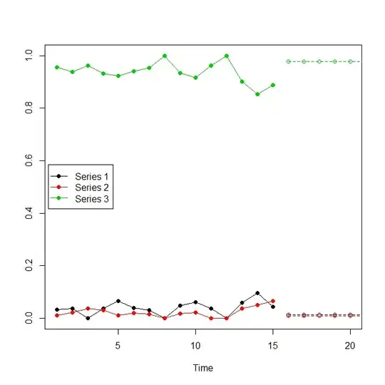
Finally, let's plot histories and forecasts:

plot(obs[,1],ylim=c(0,1),xlim=c(1,nrow(obs)+horizon),type="n",ylab="")
for ( ii in 1:ncol(obs) ) {
    lines(obs[,ii],type="o",pch=19,col=ii)
    lines(forecasts[,ii],type="o",pch=21,col=ii,lty=2)
}
legend("left",inset=.01,lwd=1,col=1:ncol(obs),pch=19,legend=colnames(obs))

EDIT: a paper on compositional time series forecasting just appeared. I haven't read it, but it may be of interest.