I am trying to use the 'density' function in R to do kernel density estimates. I am having some difficulty interpreting the results and comparing various datasets as it seems the area under the curve is not necessarily 1. For any probability density function (pdf) $\phi(x)$, we need to have the area $\int_{-\infty}^\infty \phi(x) dx = 1$. I am assuming that the kernel density estimate reports the pdf. I am using integrate.xy from sfsmisc to estimate the area under the curve.
> # generate some data
> xx<-rnorm(10000)
> # get density
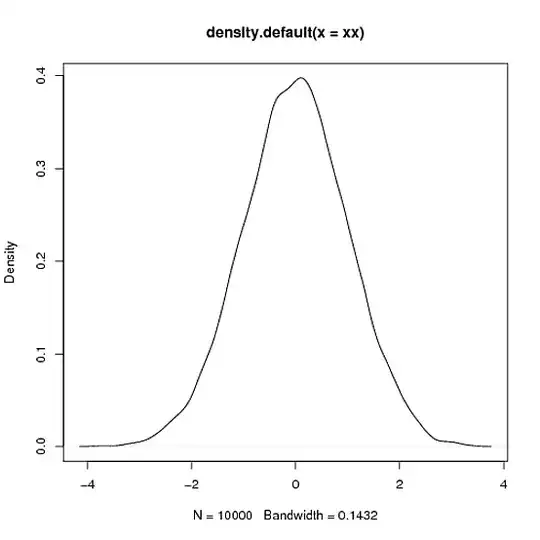
> xy <- density(xx)
> # plot it
> plot(xy)
> # load the library
> library(sfsmisc)
> integrate.xy(xy$x,xy$y)
[1] 1.000978
> # fair enough, area close to 1
> # use another bw
> xy <- density(xx,bw=.001)
> plot(xy)
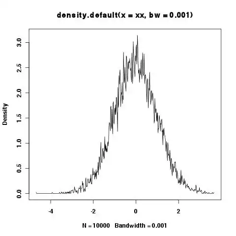
> integrate.xy(xy$x,xy$y)
[1] 6.518703
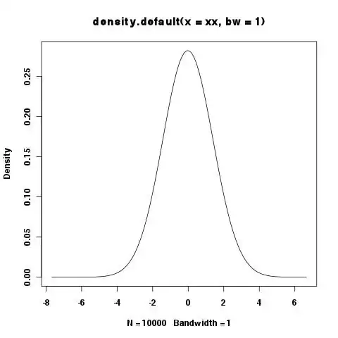
> xy <- density(xx,bw=1)
> integrate.xy(xy$x,xy$y)
[1] 1.000977
> plot(xy)
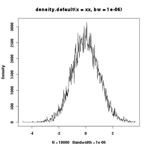
> xy <- density(xx,bw=1e-6)
> integrate.xy(xy$x,xy$y)
[1] 6507.451
> plot(xy)
Shouldn't the area under the curve always be 1? It seems small bandwidths are a problem, but sometimes you want to show the details etc. in the tails and small bandwidths are needed.
Update/Answer:
It seems that the answer below about the overestimation in convex regions is correct as increasing the number of integration points seems to lessen the problem (I didn't try to use more than $2^{20}$ points.)
> xy <- density(xx,n=2^15,bw=.001)
> plot(xy)
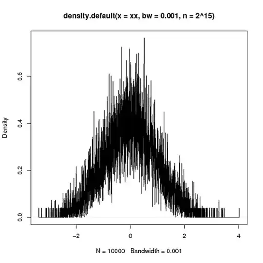
> integrate.xy(xy$x,xy$y)
[1] 1.000015
> xy <- density(xx,n=2^20,bw=1e-6)
> integrate.xy(xy$x,xy$y)
[1] 2.812398