The meaning of t-value(test statistic)? What the relation between student t distribution and t-value?

Question

I'm confused about some questions:

What the relation between student T distribution and test statistic? I would ask this question is because in wikipedia it mentions t-value below student T distribution. http://en.wikipedia.org/wiki/Student's_t-distribution#How_the_t-distribution_arises

Second, I read Baltimark's answer in (https://stats.stackexchange.com/a/295/66990). He said that ""t-value" is a generic "test statistic", not a value from a "t distribution"." Does this statement is right? In my opinion, the test statistic is the location which is certain degree of freedom and certain percentile of T distribution(for example image1) If my opinion is wrong, could anyone tell me what is wrong?

Third, I want to know where the t-value formula comes from? Why it is defined as (sample mean - null hypothesis mean)/(sqrt(sample variance/number of samples))?

Thanks a lot. I know these questions are too basic. Maybe it's because I didn't understand some fundamental ideas. Or could you recommend me some materials or books?

Thank you.

Answer 1

Q1

A $t$ value (or statistic) is the name given to a test statistic that has the form of a ratio of a departure of an estimate from some notional value and the standard error (uncertainty) of that estimate.

For example, a $t$ statistic is commonly used to test the null hypothesis that an estimated value for a regression coefficient is equal to 0. Hence the statistic is

$$ t = \frac{\hat{\beta} - 0}{\mathrm{se}_{\hat{\beta}}}$$

where the $0$ is the notional or expected value in this test, and is usually not shown.

If $\hat{\beta}$ is an ordinary least squares estimate, then the sampling distribution of the test statistic $t$ is the Student's $t$ distribution with degrees of freedom $\mathrm{df} = n - p$ where $n$ is the number of observations in the dataset/model fit and $p$ is the number of parameters fitted in the model (including the intercept/constant term).

Other statistical methods may generate test statistics that have the same general form and hence be $t$ statistics but the sampling distribution of the test statistic need not be a Student's $t$ distribution.

Q2

Baltimark's answer was in reference to the general $t$ statistic. As a test statistic we wish to assign some probability that we might see a value as extreme as the observed $t$ statistic. To do this we need to know the sampling distribution of the test statistic or derive the distribution in some way (say resampling or bootstrapping).

As mentioned above, if the estimated value for which a $t$ statistic has been computed is from an ordinary least squares, then the sampling distribution of $t$ happens to be a Student's $t$ distribution. In this specific case, you are right, you can look up the probability of observing a $t$ statistic as extreme as the one observed from a $t$ distribution of $n - p$ degrees of freedom.

So Baltimark's answer is in reference to a $t$ statistic in general whereas you are focussing on a specific application of a $t$ statistic, one for which the sampling distribution of the statistic just happens to be a Student's $t$ distribution.

Note your figure is only correct for a one-sided test. In the usual test of the null hypothesis that $\hat{\beta} = 0$ in a OLS regression, for a 95%-level test, the rejection regions — the shaded region in your figure — would be for the upper 97.5th percentile of the $t_{n-p}$ distribution, with a corresponding region in the lower tail of the distribution for the 2.5th percentile. Together the area of these regions would be 5%. this is visualised in the right hand figure below

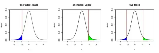
For more on this, see this recent Q&A from which I took the figure.