You could also look for a 97.5th two tailed confidence interval by using 1.25 % regions in both tails. What matter is the hypotheses involved.
In a two-tailed test you are just as happy to count large positive values (of the test statistic) as evidence against the Null as you are large negative ones. You want to spend your 5% error allowance equally in both tails hence you compute say an upper 2.5th quantile of the distribution of the test statistic and then flip the sign (as the distribution is symmetric):
> qt(0.025, 8)
[1] -2.306004
> qt(0.025, 8, lower.tail = FALSE)
[1] 2.306004
This means that you've spent 2.5% of the "error" in the lower tail and the same in the upper tail which equals the 5% "error" you were allowing.
Consider the following plots of the $t_8$ distribution (8 for the degrees of freedom as per the linked [so] question):
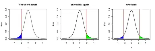
Let's also assume that this is a test on say a difference of means or a regression coefficient, the estimates of which could be positive or negative.
The left-most plot indicates the 5th (100-95th) percentile rejection region for a one-tailed test where the alternative hypothesis is that the difference of means or the regression coefficient is < 0. Large, negative values of the estimated difference of means or regression coefficient would yield large negative test statistics; values of the test statistic in the blue shaded region would constitute evidence against the null hypothesis. In this case, large positive estimates of the difference of means or regression coefficient would yield large positive $t$ values (over in the right tail of this distribution). But those large positive values shouldn't be used as evidence against the null in this one-sided test.
The same situation, only for an alternative hypothesis that the difference of means or the regression coefficient is > 0, is shown in the middle plot.
In both these plots, the critical value where the rejection region begins, is given by the 5th and 95th percentiles of the $t_8$ distribution. That value is (+/-)
> qt(0.05, 8)
[1] -1.859548
Notice this isn't as extreme as the value I calculated above for the two tailed version. This is because we can spend all the 5% uncertainty in only one or other of the tails of this distribution. We do this because we are making a stronger statement about what value we think the true difference of means of regression coefficient takes.
Often, however, we are making a less-bold statement in our alternative hypotheses; we may simply state the alternative as the difference of means or regression coefficient is not equal to 0. In that situation, large negative and positive estimates for the difference of means or the regression coefficient should be considered as evidence against the null hypothesis that the estimate = 0. If we want to maintain the same confidence level (95%) as the previous two one-tailed test, then we need to have smaller rejection regions in each tail than the rejection region in the left and middle plots. We now spend half our uncertainty allowance in the lower tail and half in the upper tail. Hence each region now contains only half the probability of the regions in the one-tailed test, but when taken together, they contain the same rejection probability.
You are free to choose the level of confidence of any of these tests, say 90th, 95th, or 99th percentile confidence. The only issue is in which tail you spend this confidence allowance and if doing a two-sided test, you spend it equally in both tails.
The R code i used to draw these plots is shown below, for reference.
png("~/tails.png", width = 900, height = 300, res = 100)
layout(matrix(1:3, ncol = 3))
x <- seq(-5, 5, by = 0.1)
dens <- dt(x, df = 8)
crit.t <- qt(0.05, 8)
## lower tail
plot(x, dens, type = "l", main = "one-tailed: lower")
abline(h = 0, col = "grey")
take <- which(x <= crit.t)
polygon(x = c(x[take], crit.t, crit.t),
        y = c(dens[take], dt(crit.t, df = 8), 0),
        col = "blue", border = "blue")
abline(v = crit.t, col = "red")
## upper tail
plot(x, dens, type = "l", main = "one-tailed: upper")
abline(h = 0, col = "grey")
take <- which(x >= -crit.t)
polygon(x = c(-crit.t, -crit.t, x[take]),
        y = c(0, dt(-crit.t, df = 8), dens[take]),
        col = "green", border = "green")
lines(x, dens, type = "l")
abline(v = -crit.t, col = "red")
## two-tailed
crit.t <- qt(0.025, 8)
plot(x, dens, type = "l", main = "two-tailed")
abline(h = 0, col = "grey")
take <- which(x <= crit.t)
polygon(x = c(x[take], crit.t, crit.t),
        y = c(dens[take], dt(crit.t, df = 8), 0),
        col = "blue", border = "blue")
take <- which(x >= -crit.t)
polygon(x = c(-crit.t, -crit.t, x[take]),
        y = c(0, dt(-crit.t, df = 8), dens[take]),
        col = "green", border = "green")
lines(x, dens, type = "l")
abline(v = c(crit.t, -crit.t), col = "red")
layout(1)
dev.off()