Predicting an output based on whether a variable is above or below a threshold

Question

I want to create a linear regression model to predict an output that uses two different coefficients based on some threshold within the data. For example: df:

Value   Temperature
8.2     70
3.2     51
5.8     54
7.2     61

and so on. For this data, I want to figure out how to make the following model:

Value = B0 + B1(HighTemp) + B2(LowTemp)

Where B1 is 0 if the temperature is below 55, and B2 is 0 is the temperature is above 55. I tried the following:

fit  = lm(Value ~ I(Temperature>55), data=df) 
fit2 = lm(Value ~ Temperature * I(Temperature>55), data=df) 

fit only gives me a coefficient for when the temperature is above 55, and fit2 gives output that I don't fully understand. I was also thinking of creating a third column, HighorLow, with an indicator variable (1 or 0) for whether or not the temperature is high or low. The I would have:

fit = lm(Value~Temperature:HighorLow, data = df)

Does anyone have any input?

Answer 1

Your last method should work, but it may be a bit clumsy to interpret because the coefficient of higher than 55 will involve adding the interaction coefficient with the temperature coefficient.

A piecewise regression may also work. You can find some tutorials here and here.

Since you use R, you may also want to look into their segmented package.

Answer 2

The theoretical model you suggest ("Value = B0 + B1(HighTemp) + B2(LowTemp)") is unidentifiable. Let's unpack that a little: There are ultimately only two possible temperature categories, high and low. Thus, you can fit two means. But you have three parameters, B0, B1 and B2. If B0 were $0$, then B1 and B2 could be the means of the two groups, but if B0 is not constrained in this manner, there are infinite sets of values that would satisfy the model. For example, imagine that the mean values for high and low were $3$ and $8$, respectively. Then you could have $0$, $3$ and $8$, or $1$, $2$ and $7$, or $-1$, $4$ and $9$, etc. There is no unique solution for the parameter estimates (see also: Qualitative variable coding in regression leads to “singularities”).

This is a common problem with categorical explanatory variables. With $k$ groups (in your case, 2), you can have only $k$ parameters. So if you have an intercept, you can have only one more parameter. There are a number of ways of coding for categorical variables that have been developed to deal with this. The most common is called "reference level coding". The mean of the reference level of your variable becomes the intercept and the other coefficient fitted is the difference between the two means. R uses by reference level coding by default; you should notice that in your first model, fit, the intercept will equal the mean of Value when Temperature is $\le 55$. This is a perfectly fine way to do it, so long as you understand the output. (I would stay away from fit2, which is a bit of a mess.)

---

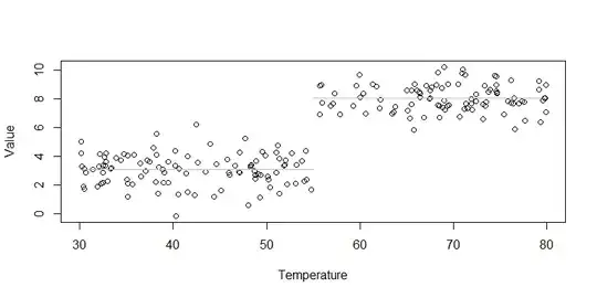
Another issue here is that you are turning a continuous variable, Temperature, into a binary indicator. This is generally a no-no; you are throwing a lot of information away and your model will be misspecified unless the true relationship looks like this:

If you believe the slope of the relationship between Temperature and Value changes at 55, you may want to fit a piecewise model, as @Penguin_Knight suggests. But you are fitting only the interaction term, which will bias the model. Consider:

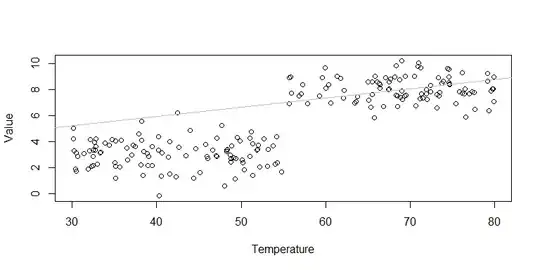
Instead, be sure to include the 'main effect' terms explicitly:

fit3a = lm(Value~Temperature+HighorLow+Temperature:HighorLow)

Or use R's shorthand, *, for an interaction that includes the main effects (these are the same):

fit3b = lm(Value~Temperature*HighorLow)
cbind(coef(fit3a),coef(fit3b))
#                               [,1]         [,2]
# (Intercept)            3.291754862  3.291754862
# Temperature           -0.005393056 -0.005393056
# HighorLow              4.787570944  4.787570944
# Temperature:HighorLow  0.005136976  0.005136976

This will yield a better specified model:

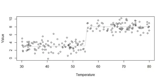
If, a-priori, you expected the slopes to be exactly 0 in both groups, you could perform a nested model test by dropping the interaction and the slope terms, and if the fit was not sufficiently worse to make you uncomfortable, you could use the test of HighorLow in the restricted model as the test of your primary hypothesis:

fit4 = lm(Value~HighorLow)
anova(fit4, fit3a)
# Model 1: Value ~ HighorLow
# Model 2: Value ~ Temperature + HighorLow + Temperature:HighorLow
#   Res.Df    RSS Df Sum of Sq      F Pr(>F)
# 1    198 207.59                           
# 2    196 207.42  2   0.17392 0.0822 0.9211
summary(fit4)
# Call:
# lm(formula = Value ~ HighorLow)
# 
# Residuals:
#     Min      1Q  Median      3Q     Max 
# -3.2365 -0.6912 -0.0097  0.7112  3.1765 
# 
# Coefficients:
#             Estimate Std. Error t value Pr(>|t|)    
# (Intercept)   3.0660     0.1004   30.54   <2e-16 ***
# HighorLow     4.9956     0.1449   34.47   <2e-16 ***
# ---
# Signif. codes:  0 ‘***’ 0.001 ‘**’ 0.01 ‘*’ 0.05 ‘.’ 0.1 ‘ ’ 1
# 
# Residual standard error: 1.024 on 198 degrees of freedom
# Multiple R-squared:  0.8572,  Adjusted R-squared:  0.8564 
# F-statistic:  1188 on 1 and 198 DF,  p-value: < 2.2e-16

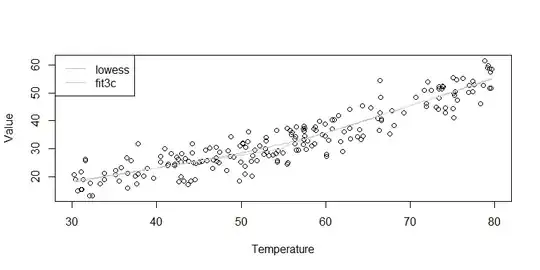
The hidden strength of using this strategy is that it will yield an appropriate fit if your data aren't like those above. The same model will not be misspecified if you need a piecewise linear model instead. Consider:

set.seed(3633)
N = 200
Temperature = runif(N, min=30, max=80)
Value       = 3 + ifelse(Temperature<55,  .5*Temperature, 0) + 
                  ifelse(Temperature>=55, 1*Temperature - 27.5, 0) +
                  rnorm(N, mean=0, sd=4)

fit3c = lm(Value~Temperature+HighorLow+Temperature:HighorLow)
summary(fit3c)
# Call:
# lm(formula = Value ~ Temperature + HighorLow + Temperature:HighorLow)
# 
# Residuals:
#    Min     1Q Median     3Q    Max 
# -9.404 -2.779 -0.111  3.335 12.421 
# 
# Coefficients:
#                        Estimate Std. Error t value Pr(>|t|)    
# (Intercept)             4.51129    2.53585   1.779   0.0768 .  
# Temperature             0.46515    0.05724   8.126 4.91e-14 ***
# HighorLow             -27.00086    4.28793  -6.297 1.95e-09 ***
# Temperature:HighorLow   0.50498    0.07698   6.560 4.69e-10 ***
# ---
# Signif. codes:  0 ‘***’ 0.001 ‘**’ 0.01 ‘*’ 0.05 ‘.’ 0.1 ‘ ’ 1
# 
# Residual standard error: 4.143 on 196 degrees of freedom
# Multiple R-squared:  0.869,  Adjusted R-squared:  0.867 
# F-statistic: 433.3 on 3 and 196 DF,  p-value: < 2.2e-16