How to reconstruct an image after performing PCA on face image dataset (eigenfaces)?

Question

I've performed PCA on face images dataset and I'm not sure how can I use the most informative principal components to show the "reduced" image.

The original image is 96*96 pixels (96*96 = 9216) and I use a sample of 70 images here (70 rows and 9216 column). We get 70 principal components (min{num of samples, num of features}=70).

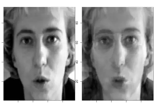
How can I re-construct a 96x96 image in order to show the eigenfaces? I want to show my students how the eigenvectors "predict" the real data.

The dataset I'm using can be downloaded here.

The code:

install.packages("foreach")

file ='C:\\I\\Love\\Data Science\\face.training.csv'
data_all = read.csv(file , stringsAsFactors=F)
dim(data_all) #7049   31

# use only 70 first images
data = data_all[1:70,]
names(data)
str(data)

# extract the images data
im.train <- data$Image
    data$Image = NULL

# each image is a vector of 96*96 pixels (96*96 = 9216).
library(foreach)
im.train <- foreach(im = im.train, .combine=rbind) %dopar% {
  as.integer(unlist(strsplit(im, " ")))
}

# im.train is a matrix of pixels 70x9216

# show picture number 2
im <- matrix(data=rev(im.train[2,]), nrow=96, ncol=96)
image(1:96, 1:96, im, col=gray((0:255)/255))

# Apply PCA
pca <- prcomp(im.train,
                 center = TRUE,
                 scale. = TRUE) ## using correlation matrix

# There are in general min(n − 1, p) informative principal components in a data set with n observations and p variables. Hence, pca$x is 70x70

# Standard deviation of each component
pca$sdev

# A numeric matrix which provides the data for the principal components analysis
pca$x
    dim(pca$x)


# The print method returns the standard deviation of each of the PCs, 
# and their rotation (or loadings), which are the coefficients of the linear combinations of the continuous variables.
print(pca)

#The summary method describe the importance of the PCs.
summary(pca)
#The first row describe again the standard deviation associated with each PC. 
#The second row shows the proportion of the variance in the data explained by each component 
#while the third row describe the cumulative proportion of explained variance. 


# plot method returns a plot of the variances (y-axis) associated with the PCs (x-axis). 
# useful to decide how many PCs to retain for further analysis. 
plot(pca, type = "l")

Answer 1

This is very similar to this previous question

Following your analysis, I use the same pca object. Looking at summary(pca) I can see that at 20 components, 90% of the variation is explained. So for demonstration purposes, that sounds like a good number to work with.

# reconstruct matrix
restr <- pca$x[,1:20] %*% t(pca$rotation[,1:20])

# unscale and uncenter the data
if(pca$scale != FALSE){
  restr <- scale(restr, center = FALSE , scale=1/pca$scale)
}
if(all(pca$center != FALSE)){
  restr <- scale(restr, center = -1 * pca$center, scale=FALSE)
}

# plot your original image and reconstructed image
par(mfcol=c(1,2), mar=c(1,1,2,1))
im <- matrix(data=rev(im.train[2,]), nrow=96, ncol=96)
image(1:96, 1:96, im, col=gray((0:255)/255))

rst <- matrix(data=rev(restr[2,]), nrow=96, ncol=96)
image(1:96, 1:96, rst, col=gray((0:255)/255))