The best way to think about the relationship between $F$, $p$, and the critical value is with a picture:
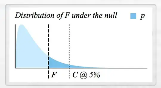
The curve here is an $F$ distribution, that is, the distribution of $F$ statistics that we'd see if the null hypothesis were true. In this diagram, the observed $F$ statistic is the distance from black dashed line to the vertical axis. The $p$ value is the dark blue area under the curve from $F$ to infinity. Notice that every value of $F$ must correspond to a unique $p$ value, and that higher $F$ values correspond to lower $p$ values.
You should notice a couple of other things about the distribution under null hypothesis:
1) $F$ values approaching zero are highly unlikely (this is not always true, but it's true for the curve in this example)
2) After a certain point, the larger the $F$ is, the less likely it is. (The curve tapers off to the right.)
The critical value $C$ also makes an appearance in this diagram. The area under the curve from $C$ to infinity equals the significance level (here, 5%). You can tell that the $F$ statistic here would result in a failure to reject the null hypothesis because it is less than $C$, that is, its $p$ value is greater than .05. In this specific example, $p=0.175$, but you'd need a ruler to calculate that by hand :-)
Note that the shape of the $F$ distribution is contingent on its degrees of freedom, which for ANOVA correspond to the # of groups (minus 1) and # of observations (minus the # of groups). In general, the overall "shape" of the $F$ curve is determined by the first number, and its "flatness" is determined by the second number. The above example has a $df_1 = 3$ (4 groups), but you'll see that setting $df_1 = 2$ (3 groups) results in a markedly different curve:
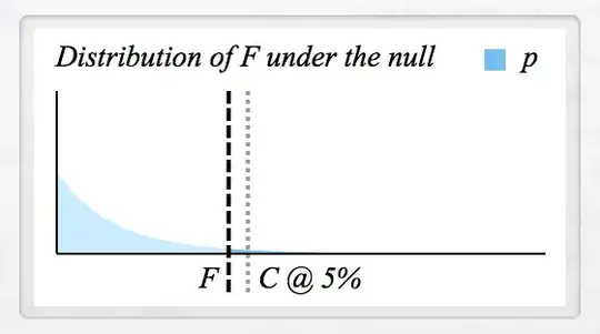
You can see other variants of the curve on Mr. Wikipedia Page. One thing worth noting is that because the $F$ statistic is a ratio, large numbers are uncommon under the null hypothesis, even with large degrees of freedom. This is in contrast to $\chi^2$ statistics, which are not divided by the number of groups, and essentially grow with the degrees of freedom. (Otherwise $\chi^2$ is analogous to $F$ in the sense that $\chi^2$ is derived from normally distributed $z$ scores, whereas $F$ is derived from $t$-distributed $t$ statistics.)
That's a lot more than I meant to type, but I hope that covers your questions!
(If you're wondering where the diagrams came from, they were automatically generated by my desktop statistics package, Wizard.)