What kind of residuals and Cook's distance are used for GLM?

Question

Does anybody know what the formula for Cook's distance is? The original Cook's distance formula uses studentized residuals, but why is R using std. Pearson residuals when computing the Cook's distance plot for a GLM. I know that studentized residuals are not defined for GLMs, but how does the formula to compute Cook's distance look like?

Assume the following example:

numberofdrugs <- rcauchy(84, 10)
healthvalue <- rpois(84,75)
test <- glm(healthvalue ~ numberofdrugs, family=poisson)
plot(test, which=5) 

What is the formula for Cook's distance? In other words, what is the formula to compute the red dashed line? And where does this formula for standardized Pearson residuals come from?

Answer 1

If you take a look at the code (simple type plot.lm, without parenthesis, or edit(plot.lm) at the R prompt), you'll see that Cook's distances are defined line 44, with the cooks.distance() function. To see what it does, type stats:::cooks.distance.glm at the R prompt. There you see that it is defined as

(res/(1 - hat))^2 * hat/(dispersion * p)

where res are Pearson residuals (as returned by the influence() function), hat is the hat matrix, p is the number of parameters in the model, and dispersion is the dispersion considered for the current model (fixed at one for logistic and Poisson regression, see help(glm)). In sum, it is computed as a function of the leverage of the observations and their standardized residuals. (Compare with stats:::cooks.distance.lm.)

For a more formal reference you can follow references in the plot.lm() function, namely

Belsley, D. A., Kuh, E. and Welsch, R. E. (1980). Regression Diagnostics. New York: Wiley.

Moreover, about the additional information displayed in the graphics, we can look further and see that R uses

plot(xx, rsp, ...                    # line 230
panel(xx, rsp, ...)                  # line 233
cl.h <- sqrt(crit * p * (1 - hh)/hh) # line 243
lines(hh, cl.h, lty = 2, col = 2)    #
lines(hh, -cl.h, lty = 2, col = 2)   #  

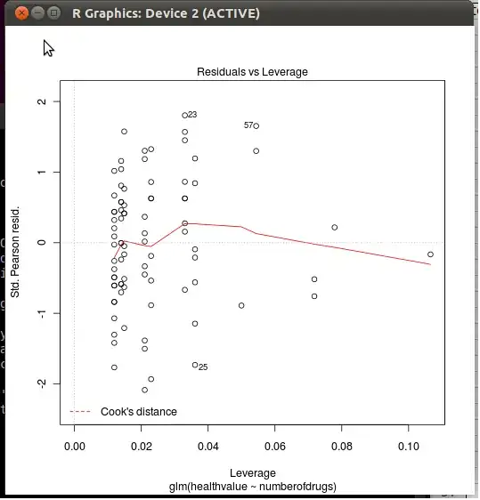
where rsp is labeled as Std. Pearson resid. in case of a GLM, Std. residuals otherwise (line 172); in both cases, however, the formula used by R is (lines 175 and 178)

residuals(x, "pearson") / s * sqrt(1 - hii)

where hii is the hat matrix returned by the generic function lm.influence(). This is the usual formula for std. residuals:

$$rs_j=\frac{r_j}{\sqrt{1-\hat h_j}}$$

where $j$ here denotes the $j$th covariate of interest. See e.g., Agresti Categorical Data Analysis, §4.5.5.

The next lines of R code draw a smoother for Cook's distance (add.smooth=TRUE in plot.lm() by default, see getOption("add.smooth")) and contour lines (not visible in your plot) for critical standardized residuals (see the cook.levels= option).