Why does SAS PROC GLIMMIX give me VERY different random slopes than glmer (lme4) for a binomial glmm

Question

I am a user more familiar with R, and have been trying to estimate random slopes (selection coefficients) for about 35 individuals over 5 years for four habitat variables. The response variable is whether a location was "used" (1) or "available" (0) habitat ("use" below).

I am using a Windows 64-bit computer.

In R version 3.1.0, I use the data and expression below. PS, TH, RS, and HW are fixed effects (standardized, measured distance to habitat types). lme4 V 1.1-7.

str(dat)
'data.frame':   359756 obs. of  7 variables:
 $ use     : num  1 1 1 1 1 1 1 1 1 1 ...
 $ Year    : Factor w/ 5 levels "1","2","3","4",..: 4 4 4 4 4 4 4 4 3 4 ...
 $ ID      : num  306 306 306 306 306 306 306 306 162 306 ...
 $ PS: num  -0.32 -0.317 -0.317 -0.318 -0.317 ...
 $ TH: num  -0.211 -0.211 -0.211 -0.213 -0.22 ...
 $ RS: num  -0.337 -0.337 -0.337 -0.337 -0.337 ...
 $ HW: num  -0.0258 -0.19 -0.19 -0.19 -0.4561 ...

glmer(use ~  PS + TH + RS + HW +
     (1 + PS + TH + RS + HW |ID/Year),
     family = binomial, data = dat, control=glmerControl(optimizer="bobyqa"))

glmer gives me parameter estimates for the fixed effects that make sense to me, and the random slopes (which I interpret as selection coefficients to each habitat type) also make sense when I investigate the data qualitatively. The log-likelihood for the model is -3050.8.

However, most research in animal ecology do not use R because with animal location data, spatial autocorrelation can make the standard errors prone to type I error. While R uses model-based standard errors, empirical (also Huber-white or sandwich) standard errors are preferred.

While R does not currently offer this option (to my knowledge - PLEASE, correct me if I am wrong), SAS does - although I do not have access to SAS, a colleague agreed to let me borrow his computer to determine if the standard errors change significantly when the empirical method is used.

First, we wished to ensure that when using model-based standard errors, SAS would produce similar estimates to R - to be certain that the model is specified the same way in both programs. I don't care if they are exactly the same - just similar. I tried (SAS V 9.2):

proc glimmix data=dat method=laplace;
   class year id;
   model use =  PS TH RS HW / dist=bin solution ddfm=betwithin;
   random intercept PS TH RS HW / subject = year(id) solution type=UN;
run;title;

I also tried various other forms, such as adding lines

random intercept / subject = year(id) solution type=UN;
random intercept PS TH RS HW / subject = id solution type=UN;

I tried without specifying the

solution type = UN,

or commenting out

ddfm=betwithin;

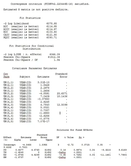
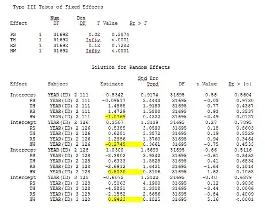
No matter how we specify the model (and we have tried many ways), I cannot get the random slopes in SAS to remotely resemble those output from R - even though the fixed effects are similar enough. And when I mean different, I mean that not even the signs are the same. The -2 Log Likelihood in SAS was 71344.94.

I can't upload my full dataset; so I made a toy dataset with only the records from three individuals. SAS gives me output in a few minutes; in R it takes over an hour. Weird. With this toy dataset I'm now getting different estimates for the fixed effects.

My question: Can anyone shed light on why the random slopes estimates might be so different between R and SAS? Is there anything I can do in R, or SAS, to modify my code so that the calls produce similar results? I'd rather change the code in SAS, since I "believe" my R estimates more.

I'm really concerned with these differences and want to get to the bottom of this problem!

My output from a toy dataset that uses only three of the 35 individuals in the full dataset for R and SAS are included as jpegs.

---

EDIT AND UPDATE:

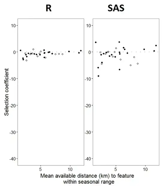
As @JakeWestfall helped discover, the slopes in SAS do not include the fixed effects. When I add the fixed effects, here is the result - comparing R slopes to SAS slopes for one fixed effect, "PS", between programs: (Selection coefficient = random slope). Note the increased variation in SAS.

Answer 1

It appears that I shouldn't have expected the random slopes to be similar between packages, according to Zhang et al 2011. In their paper On Fitting Generalized Linear Mixed-effects Models for Binary Responses using Different Statistical Packages, they describe:

Abstract:

The generalized linear mixed-effects model (GLMM) is a popular paradigm to extend models for cross-sectional data to a longitudinal setting. When applied to modeling binary responses, different software packages and even different procedures within a package may give quite different results. In this report, we describe the statistical approaches that underlie these different procedures and discuss their strengths and weaknesses when applied to fit correlated binary responses. We then illustrate these considerations by applying these procedures implemented in some popular software packages to simulated and real study data. Our simulation results indicate a lack of reliability for most of the procedures considered, which carries significant implications for applying such popular software packages in practice.

I hope @BenBolker and team will consider my question as a vote for R to incorporate empirical standard errors and Gauss-Hermite Quadrature capability for models with several random slope terms to glmer, as I prefer the R interface and would love to be able to apply some further analyses in that program. Happily, even while R and SAS do not have comparable values for random slopes, the overall trends are the same. Thanks all for your input, I really appreciate the time and consideration that you put into this!

Answer 2

A mixture of an answer and commentary/more questions:

I fitted the 'toy' data set with three different optimizer choices. (*Note 1: it would probably be more useful for comparative purposes to make a small data set by subsampling from within every year and id, rather than by subsampling the grouping variables. As it is, we know that the GLMM won't perform particularly well with such a small number of grouping variable levels. You can do this via something like:

library(plyr)
subdata <- ddply(fulldata,c("year","id"),
    function(x) x[sample(nrow(x),size=round(nrow(x)*0.1)),])

Batch fitting code:

Ntoy <- readRDS("Newton_toy.RDS")
library(lme4)
fitfun <- function(opt) {
    tt <- system.time(fit1 <- glmer(use ~  ps + th + rs + hw +
                                    (1 + ps + th + rs + hw |id/year),
                                    family = binomial, data = Ntoy,
                                    control=glmerControl(optimizer=opt),
                                    verbose=100))
    return(list(time=tt,fit=fit1))
}

opts <- c("nloptwrap","nlminbwrap","bobyqa")
## use for() instead of lapply so we can checkpoint more easily
res <- setNames(vector("list",length(opts)),opts)
for (i in opts) {
    res[[i]] <- fitfun(i)
    save("res",file="Newton_batch.RData")
}

Then I read in the results in a new session:

load("Newton_batch.RData")
library(lme4)

Elapsed time and deviance:

cbind(time=unname(sapply(res,function(x) x$time["elapsed"])),
          dev=sapply(res,function(x) deviance(x$fit)))
##                time      dev
## nloptwrap  1001.824 6067.706
## nlminbwrap 3495.671 6068.730
## bobyqa     4945.332 6068.731

These deviances are considerably below the deviance reported by the OP from R (6101.7), and slightly below the ones reported by the OP from SAS (6078.9), although comparing deviances across packages is not always sensible.

I was indeed surprised that SAS converged in only about 100 function evaluations!

Times range from 17 minutes (nloptwrap) to 80 minutes (bobyqa) on a Macbook Pro, consistent with the OP's experience. Deviance is a bit better for nloptwrap.

round(cbind(sapply(res,function(x) fixef(x$fit))),3)
##             nloptwrap nlminbwrap bobyqa
## (Intercept)    -5.815     -5.322 -5.322
## ps             -0.989      0.171  0.171
## th             -0.033     -1.342 -1.341
## rs              1.361     -0.140 -0.139
## hw             -2.100     -2.082 -2.082

Answers appear quite different with nloptwrap -- although the standard errors are quite large ...

round(coef(summary(res[[1]]$fit)),3)
##             Estimate Std. Error z value Pr(>|z|)
## (Intercept)   -5.815      0.750  -7.750    0.000
## ps            -0.989      1.275  -0.776    0.438
## th            -0.033      2.482  -0.013    0.989
## rs             1.361      2.799   0.486    0.627
## hw            -2.100      0.490  -4.283    0.000

(code here gives some warnings about year:id that I should track down)

To be continued ... ?