Intervention Analysis - Pulse over several periods

Question

I have a couple weekly time series and an intervention occurred over several weeks and then for some, after a period of no intervention, began again. So, the pattern is off for a period of weeks, then on for a period of weeks, then off for a period of weeks and perhaps on again.

The image below tries to show the possible patterns:

When there is a single pulse, then as discussed here it is pretty simple to code the intervention as a pulse (1 or that period and zero elsewhere) and code the transfer function as one of several shapes - e.g. only effecting a single period (the pulse), a permanent level shift (a step) or perhaps with a lasting (but decaying) effect (a pulse but with decay transfer function).

In the situation described here though, is there the same flexibility or do we really only have the option to code the interventions as 10 separate interventions (for the top series) or 5 separate ones for the bottom series and only allow the intervention to effect the single period? I am not sure how to have any of the "pulses" have a decaying effect because where does one start and the other stop?

In my reading thus far for this type of analysis I have seen the pulse and step but nothing like this, where there is an "on" for a period of time, then "off" and then on again (maybe).

Answer 1

Lets say you have a time series data 42 observations. Observation 7 to 13 have step(level shift) intervention and observations 29 to 35 have step intervention of 5 units. The remainder observations are 0. As an example, see below chart for simulated data with actual and actual + error.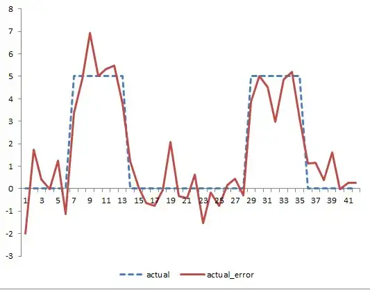

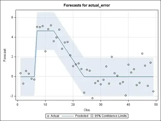
If you would like to model this data as a intervention analysis using arima transfer function, you simply need to create a dummy coded variable with 1's for 7 to 13 and 1's for 29 to 35 and pass this is a step intervention in ARIMAX model. I don't know how to use R for transfer function modeling, so I used SAS. See below the actual and predicted data. The ARIMAX approximated the data very well. See below the SAS code that I used to create the data and as well as the ARIMAX.

If your second intervention has a first intervention has a decaying effect, all you need to do is create a second intervention variable at the end of first step function and code it appropriately.

Hopefully this helped.

data temp;
    input actual @@;
    error = rand("NORMAL");
    datalines;
0 0 0 0 0 0 5
5 5 5 5 5 5 0
0 0 0 0 0 0 0
0 0 0 0 0 0 0
5 5 5 5 5 5 5
0 0 0 0 0 0 0
;
run;

data temp;
    set temp;
      actual_error = actual+error; *add random error;

      if 7 <= _n_ <= 14 or 29 <= _n_ <= 35 then step = 1; * First Intervention step;
            else step = 0;

run;

ods graphics on;
proc arima data = temp plots = all;
    identify var=actual_error crosscorr = (step); 
     estimate input = (step) method = ml outest = mm1; /*Estimate Model using Transfer Function*/
     forecast out = out1 lead = 0;
run;
ods graphics off;

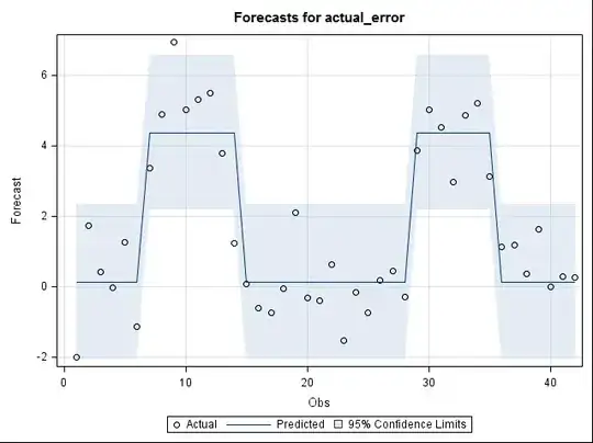
EDIT: as b_miner would like to know how to model this with temporary level shift with a linear decay, I have modified the example. I have shown only the first level shift, the second level shift could be easily added. If you are looking for a decay other than a linear decay then it is fairly easy to do, just use a step+gradual permanent decay function using transfer function. Intervention modeling is more of an art than science. You assume a shape, test the hypothesis, if acceptable move on else change the shape. Intervention modeling is deterministic in nature. If you are interested in learning more about transfer function modeling/intervention detection, I would highly recommend Forecasting-Dynamic-Regression-Models-Pankratz. This text has all the different types of intervention models possible, in addition to transfer function modeling.

Hope this helps.

data temp;
    input actual @@;
    error = rand("NORMAL");
    datalines;
0 0 0 0 0 0 5
5 5 5 5 5 5 4.1
4 3.5 3 2.5 2 1.75 1.25
0.75 0.25 0 0 0 0 0
0 0 0 0 0 0 0
0 0 0 0 0 0 0
0 0 0 0 0 0 0
;
run;

data temp;
    set temp;
    retain ramp 0;
      actual_error = actual+error; *add random error;

      if 7 <= _n_ <= 13 then step = 1;
            else step = 0;


      if 14 <= _n_ <= 23  then do;
            step = (_n_ - 24)/(13-24); 

      end;

run;



ods graphics on;
proc arima data = temp plots = all;
    identify var=actual_error crosscorr = (step); 
     estimate input = (step) method = ml outest = mm1; /*Estimate Model using Transfer Function*/
     forecast out = out1 lead = 0;
run;
ods graphics off;