Compute mode of a quadratic regression with confidence intervals

Question

I have a quadratic regression y against x and I'm interested in the value x where y is the maximum (ymax->x). I can compute x(ymax) but I'm also interested in the standard error or confidence interval of x(ymax) to get x(ymax) +/- standard error or, respectively, lower and upper xmax confidence interval.

One solution could be to use bootstrap methods and computing new estimates of beta but the real data I have is large and needs one hour to compute the model (mixed model with variance-covariance structure).

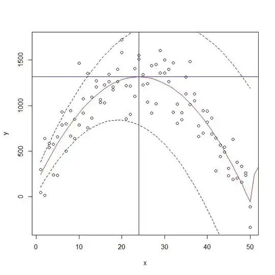
Another possibility would be to use the standard errors of the betas to compute a confidence band and to find the cutting points of the horizontal through maximum of the curve and the upper "confidence curve" (see below). But I'm not sure if this method is a valid way to get confidence interval.

Is there anyone who can give me some advice how to cope with this?

Thanks in advance.

---

# simulate data set
b0 <- 100
b1 <- 100
b2 <- -2
(x <- rep(1:50,2))
(y <- b0 + b1*x + b2*x^2 + rnorm(length(x),0,200))

# fit model
fit <- lm(y~x + I(x^2))
summary(fit)

# visualize
plot(y~x)
lines(fitted(fit), col="red")

# retrieve coefficients
beta <- fit$coef

# build function for optimization
f1 <- function(x) sum(beta * c(1,x,x^2))

# compute xmax
(xymax <- optimize(f1,interval=c(0,50), maximum=TRUE))

# add line at xmax
# add line at xmax
abline(v=xymax$max, col="blue")
abline(h=xymax$obj, col="blue")

# compute confidence band
cilbeta <- beta - qnorm(0.975,0,1)*summary(fit)$coef[,"Std. Error"]
ciubeta <- beta + qnorm(0.975,0,1)*summary(fit)$coef[,"Std. Error"]
f2 <- function(x) { sum(c(1,x,x^2)*cilbeta) }
f3 <- function(x) { sum(c(1,x,x^2)*ciubeta) }
# curve(f2,from=1,to=50)  does not work !!
ycil = c()
yciu = c()
for (i in 1:50) {
    ycil <- c(ycil,f2(i))
    yciu <- c(yciu,f3(i))
}
lines(1:50,ycil, lty=2)
lines(1:50,yciu, lty=2)

# cutting points between upper "confidence curve" horizontal line
# through y.max


# x.max = -b2/(2b3) = -0.5*b2/b3
# var(x.max) = 0.5^2*var(b2/b3)
# var.b23 = b2^2/b3^2*[var(b2)/b2^2 -2*cov(b2,b3)/(b2*b3) + var(b3)/b3^2]
(var.b23 <- coef0[2]^2/coef0[3]^2*(vcov0[2,2]/coef0[2]^2 
            -2*vcov0[2,3]/(coef0[2]*coef0[3]) + vcov0[3,3]/coef0[3]^2
            )
        )
(var.xmax <- (-0.5)^2*var.b23)
(se.xmax <- sqrt(var.xmax))
# confidence interval
paste(formatC(x.max,digits=2,format="f")," ("
      , formatC(x.max-2*se.xmax,digits=2, format="f"),"-"
      , formatC(x.max+2*se.xmax,digits=2,format="f"),")"
      , sep=""
      )
# [1] "24.77 (24.12-25.42)"

Answer 1

The mode of the quadratic function $$ b_1 + b_2 x + b_3 x^2 $$ is at $M = -b_2/(2 b_3)$ as long as $b_3$ is negative. (Compare with the solution in your code).

The standard deviation of M can be derived by bootstrap or analytically:

In http://www.stat.cmu.edu/~hseltman/files/ratio.pdf you can find an approximation of the variance of a ratio of two correlated random variables. (Note that the exact variance seems to be inherently complicated, even in the bivariate normal case.) So just replace the expectations, variances and covariances in the last formula of the article by the estimates from the regression.