7

I am currently trying to fit distributions to some heavy tailed data-set (see the data set below) and have a hard time producing good results:

v1 <- c(11.87,14.04,11.86,179.88,13.09,14.68,13.54,32.25,54.52,66.28,15.16,39.83,89.81,116.87,298.94,427,6249.42,3334.9,4503.93,4933.9,15.72,12.33,13.64,15.12,47.86,12.3,12.79,12.34,14.44,12.17,120.17,12.82,13.07,47.48,13.72,12.19,30.48,129.16,191.41,282.96,1076.53,4354.01,7882.12,12.45,13.9,12.12,16.63,12.26,12.01,17.87,12.62,11.81,12.68,12.33,12.04,15.64,12,13.1,62.44,13.21,13.28,12.99,13.52,23.47,13.36,11.81,11.86,13.74,58.72,12.72,12.02,11.92,44.75,77.96,23.53,11.81,23.46,12.52,29.47,12.31,12.54,11.86,12.42,11.89,11.94,12.44,13.48,12.37,16.3,11.93,28.1,18.85,11.96,11.94,18.64,11.79,12.1,13.82,29.8,19.6,11.79,12.77,11.77,14.92,20.59,12.24,19.39,12.79,20.97,13.01,32.79,12.73,24.56,11.92,13.08,12.41,14.46,27.26,25.51,13.8,32.35,15.32,27.82,15.26,13.71,29.8,12.72,14.7,12.28,14.55,12.13,12.86,18.36,36.18,12.1,14.56,29.34,11.82,12,12.21,27.98,17.86,14.13,13.45,17.53,14,13.08,12.23,14.94,14.12,13.19,20.14,40.22,21.19,14.46,35.38,14.89,31.77,3057.58,12.86,12.15,20.52,132.7,17.5,31.34,15.27,13.45,15.32,24.75,12.45,13.45,29.4,13.82,13.48,83.84,100.4,12.78,31.58,16.59,12.51,59.34,66.09,232.43,12.74,12.21,73.53,109.48,13.53,17.65,87.09,18.93,12.43,12.32,15.55,14.1,12.15,12.43,11.82,12.87,12.28,140,240.49,12.76,25.97,13.6,18.32,117.4,242.05,13.94,111,161.53,247.33,13.51,15.49,65.64,14.27,35.17,11.83,30.21,29.14,12.53,11.76,14.08,49.06,212.09,258.35,13,13.74,29.08,60.23,12.16,142.66,202.93,74.79,12.88,27.48,48.91,64.79,49.25,224.59,299.4,29.24,68.88,15.12,34.8,23.68,43.55,12.4,17.61,18.1,15.15,11.92,14.17,13.45,14.51,44.46,14.24,34.15,258.84,12.75,12.77,34.44,13.12,22.49,53.46,14.96,13.75,11.77,16.2,12.52,12.19,17.69,34.83,13.25,12.39,29.59,56.69,82.38,12.13,27.69,15.12,50.21,68.42,16.84,14.96,11.81,15.53,168.74,797.01,52.84,67.02,15.83,167.27,240.05,12.03,48.64,30.45,28.81,54.1,17.73,33.99,19.93,37.21,35.3,122.36,44.94,15.2,26.46,217.48,257.06,14.69,13.22,55.8,26.95,55.05,16.71,44.58,20.71,14.24,41.69,58.3,108.43,137.71,13.89,19.53,46.72,22.45,36.93,20.72,17.39,15.32,28.83,16.34,26.04,44.12,17.84,14.23,14.17,13.63,13.12,12.91,12.72,36.33,18.25,14.06,14.67,27.51,18.38,12.69,14.14,16.19,11.87,12.26,31.92,14.09,19.07,32.24,19.29,34.24,21.39,13.05,17.57,5651.61,6635.33,1666.81,6692.4,2161.37,15.63,37.85,61.85,68.92,252.31,16.45,28.21,57.45,93.8,70.53,178.19,239.22,270.67,419.6,11.93,11.88,14.38,51.44,54.91,81.9,112.63,3911.01,8625.72,9144.85,11.9,19.59,39.06,3153.42,8628.67,17.58,12.7,11.91,17.08,11.92,18.83,12.09,13.19,14.02,11.74,42.91,225.66,257.56,18.97,58.93,150.21,249.29,262.74,20.67,48.07,239.44,283.07,777.53,866.46,2570.59,5306.95,7773.85,8706.43,8730.16,21.43,86.28,12.22,103.45,120.04,197.63,502.12,580.07,19.02,18.98,12.3,13.49,50.26,76.13,14.69,44.07,73.74,180.95,13.37,15.37,58.62,60.12,228.92,251.56,268.03,11.77,16.83,50.36,63.02,107.3,234.99,261.7,18.09,58.17,75.96,220.08,250.4,16.36,14.1,61.36,140.59,278.06,417.68,797.12,1633.51,3911.59,3463.77,32.29,59.93,17.8,70.88,88.52,244.83,282.94,312.01,658.95,828.67,15.23)

I tried to fit a generazlied extreme value and a skewed student-t distribution to it:

library(fExtremes)

# generalized extreme value distribution
empFit <- gevFit(v1)
coefs <- slot(empFit, 'fit')$par.ests
qqplot(v1, rgev(1e4, xi = coefs['xi'], mu = coefs['mu'], beta = coefs['beta']),ylim=c(0,1e4))
abline(0,1)


# skewed-student t
empFit <- sstdFit(v1)
vpars <- empFit$estimate
qqplot(v1, rsstd(1e4,vparas[1],vparas[2],vparas[3],vparas[4]),ylim=c(0,1e4))
abline(0,1)

The qqplots do not look very promising. The gev-distribution is completely off and the student-t is not capable of capturing the tails very well.

I would really appreciate any help / comments in this regard as I am no expert in heavy-tailed distributions.

I already tried to just fit the values above the .95 quantile with a generalized pareto and the remaining part with something else. But I am not sure whether this is a good approach to take.

Another observation: Also tried out some other distributions and packages but very often find that the optimizers for fitting the distribution have a hard time in dealing with the likelihood (that is why I also question the parameters obtained in the above one examples).
kjetil b halvorsen
  • 63,378
  • 26
  • 142
  • 467
user3777456
  • 346
  • 3
  • 6
  • 1
    What are these data? The fact that the data are heavy-tailed doesn't justify the use of the GEV distribution. Why did you consider the GEV distribution for these data? – QuantIbex Jun 26 '14 at 07:37
  • 1
    This are basically spikes in electricity price-timeseries. So, they were filtered (by some 3-sigma algorithm). There is no specific reason for chossing the GEV. Tried out other distributions as well but didnt work out that well. I would be glad if you had some suggestions in that regard? – user3777456 Jun 26 '14 at 07:54
  • 2
    The GEV distribution is suitable to model data that correspond to maxima of some observations, e.g., the maximum hourly rain over a week, which doesn't seem to be the case here since your data is a filtered price series, not the series of maximum prices over some extended periods of time (e.g., a week/month). What filter did you apply? Does `v1` contain values larger that the mean plus three standard deviations? – QuantIbex Jun 26 '14 at 08:19
  • Good point with the GEV distribution. For filtering I used a recursive procedure: Remove all values larger than mean + 3*standard deviation. Repeat this step until the change in the variance of the data-set does not change considerably (or not spikes are found anymore). Yes, mean(v1) + 3*sd(v1) = 4200. And there are values in the range of 10 000. – user3777456 Jun 26 '14 at 08:26
  • 1
    Your data *is* highly skew but the extreme tail seems to be short, not long. There's 5 values between 8625 and 9145, which is only a tiny amount of variation (9145/8625 is only 1.06). Look at the reciprocal of `v1` and you can discern a number of interesting features, including a large spike around 1/250 (because, again, there's a lot more values concentrated relatively near 250 than you'd expect with a typical heavy-tailed distribution). – Glen_b Jun 26 '14 at 10:21
  • 3
    (ctd) ... It looks to me like a mixture of several not-so-heavy-tailed distributions may do better, or perhaps something roughly like a Pareto to fit the lower end and some much-shorter-tailed components near 250 and 8700-ish, and possibly a couple of lower ones as well. – Glen_b Jun 26 '14 at 10:28
  • Interesting you suggest looking at the reciprocal of the data. Is that some common thing for analyzing heavy-tailed data? How would you proceed in deciding on how many distributions how the data is "split"? I guess one could just decide for the upper 10 or 5 percent quantile. At least theoretically one could determine the "cutoff-point" between the distributions by maximum-liklihood, too. Will most likely try to post some results tomorrow. – user3777456 Jun 26 '14 at 13:36

4 Answers4

3

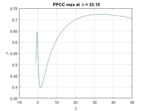
I applied Tukey-Lambda PPCC to your data to get the following plot: enter image description here

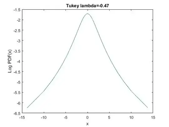
You see the local max at $\lambda=-0.47$, which implies heavier tails than normal distribution. For normal it's 0.14 and for Cauchy it's -1. So, if you go with this view, then your data's tail is not as "fat" as Cauchy's, but much fatter than normal.

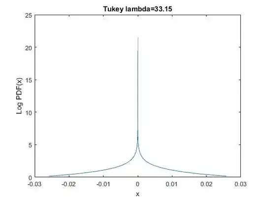
However the global max is at $\lambda=33.17$

I drew the Tukey lambda for the above two maxima here: enter image description here enter image description here

So, you have two very different views of the distribution. One is fat tailed, the other one's very convex.

I think that the convex distribution is the better fit. Cauchy and other fat tailed ones are not a good fit here, go for these weird distributions like in my last plot.

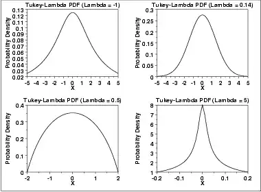
Here's how Tukey Lambda distribution looks like for some $\lambda$. enter image description here

I use this tool to gauge the shape of my data.

Aksakal
  • 55,939
  • 5
  • 90
  • 176
2

your data set is really very long-tailed. Consider making 1st some tests on less extreme data (to check this look e.g. to sampling kurtosis). L-moments are not suited for very-very-long tail data, e.g. for Cauchy distribution not all L-moments exist.

Bye Stephan

user32038
  • 409
  • 3
  • 10
  • Thanks. Also tried to fit some distributions by the method of L-moments and get thrown back "L-moments invalid"-messages. Does not seem to help a lot here unfortunately. What do you think about splitting the data-set in two? Like a log-normal and a gev for the tail? I have to say though, that this data-set is basically already the "tail" of some larger data set which has been filtered by some naive 3-sigma-algorithm. So ideally, I did want to model it by just one type of distribution. – user3777456 Jun 26 '14 at 07:51
  • What about partial L-moments as in http://www.tbm.tudelft.nl/fileadmin/Faculteit/CiTG/Over_de_faculteit/Afdelingen/Afdeling_Waterbouwkunde/sectie_waterbouwkunde/people/personal/gelder/publications/citations/doc/citatie109.pdf – kjetil b halvorsen Sep 15 '15 at 16:24
1

One way to do this is to construct an L-moment diagram with your data. There in an R package (with full manual) at http://cran.r-project.org/web/packages/lmom/index.html.

The L-moment diagram will plot the L-skewness and L-kurtosis of your data on a chart and show how different distribution-types would appear on that same chart so you can try to select a known distribution.

hydrologist
  • 722
  • 1
  • 5
  • 20
  • Hi there, thanks a lot for your answer! Could you elaborate a bit on why I should make use of those l-moments instead of just fitting heavy-tailed distributions and observing qq-plots? Also, in the end I will still have to use some heavy-tailed distribution and fit it to the data as before. So I do not see how this diagram could help exactly? Thanks in advance! – user3777456 Jun 26 '14 at 07:23
  • 1
    Yes. The problem here is that you don't know what distribution to fit - the L-moment diagram could help you with this, and provide a first estimate of the parameters. I can't see all of your dataset (can you dropbox it)? – hydrologist Jun 26 '14 at 08:20
  • I can share on dropbox. But cant you just select it in the above message? I specifically put it there so you could reproduce it easily. – user3777456 Jun 26 '14 at 08:27
1

experimented a bit with a mixture of distributions but am still far from a satisfying result..

Data-set is the same as above (v1). The maximum-likelihood function for the pareto is given by:

 pareto.MLE <- function(X)
 {
 n <- length(X)
 m <- min(X)
 a <- n/sum(log(X)-log(m))
 return( c(m,a) ) 
 }

Now, I fit the upper tail of the data-set separately:

pquant <- .95

idx <- which(v1>quantile(v1,pquant))
v1a <- v1[idx]
vpars1 <- pareto.MLE(v1a)

qqplot(v1a, rpareto(1e4, vpars1[1],vpars1[2]),ylim=c(0,1e4))
abline(0,1)

v1b <- v1[-idx]
vpars2 <- pareto.MLE(v1b)

qqplot(v1b, rpareto(1e4, vpars2[1],vpars2[2]))
abline(0,1)

v3 <- c(rpareto(1e5*.95, vpars2[1],vpars2[2]),rpareto(1e5*.05,vpars1[1],vpars1[2]))
qqplot(v1,v3,ylim=c(0,1e4))
abline(0,1)

The qq-plots look very poor. Furthermore, whenever fitting the upper tail, I get ridicously high values with a too high probability.. The remaining part of the distributions is not fitted well, too.. I would welcome any further suggestions in that regard!

Another question: What kind of "tail-measures" for evaluating the goodness of the fit for the tail are sensible? RMSE does not seem to be the right choice here? I still ony judge qualitatively by insepcting qq-plots.

Best

user3777456
  • 346
  • 3
  • 6