What is the difference between "loadings" and "correlation loadings" in PCA and PLS?

Question

One common thing to do when doing Principal Component Analysis (PCA) is to plot two loadings against each other to investigate the relationships between the variables. In the paper accompanying the PLS R package for doing Principal Component Regression and PLS regression there is a different plot, called the correlation loadings plot (see figure 7 and page 15 in the paper). The correlation loading, as it is explained, is the correlation between the scores (from the PCA or PLS) and the actual observed data.

It seems to me that loadings and correlation loadings are pretty similar, except that they are scaled a bit differently. A reproducible example in R, with the built in data set mtcars is as follows:

data(mtcars)
pca <- prcomp(mtcars, center=TRUE, scale=TRUE)

#loading plot
plot(pca$rotation[,1], pca$rotation[,2],
     xlim=c(-1,1), ylim=c(-1,1),
     main='Loadings for PC1 vs. PC2')

#correlation loading plot
correlationloadings <- cor(mtcars, pca$x)
plot(correlationloadings[,1], correlationloadings[,2],
     xlim=c(-1,1), ylim=c(-1,1),
     main='Correlation Loadings for PC1 vs. PC2')

What is the difference in interpretation of these plots? And which plot (if any) is best to use in practice?

Answer 1

Warning: R uses the term "loadings" in a confusing way. I explain it below.

Consider dataset $\mathbf{X}$ with (centered) variables in columns and $N$ data points in rows. Performing PCA of this dataset amounts to singular value decomposition $\mathbf{X} = \mathbf{U} \mathbf{S} \mathbf{V}^\top$. Columns of $\mathbf{US}$ are principal components (PC "scores") and columns of $\mathbf{V}$ are principal axes. Covariance matrix is given by $\frac{1}{N-1}\mathbf{X}^\top\mathbf{X} = \mathbf{V}\frac{\mathbf{S}^2}{{N-1}}\mathbf{V}^\top$, so principal axes $\mathbf{V}$ are eigenvectors of the covariance matrix.

"Loadings" are defined as columns of $\mathbf{L}=\mathbf{V}\frac{\mathbf S}{\sqrt{N-1}}$, i.e. they are eigenvectors scaled by the square roots of the respective eigenvalues. They are different from eigenvectors! See my answer here for motivation.

Using this formalism, we can compute cross-covariance matrix between original variables and standardized PCs: $$\frac{1}{N-1}\mathbf{X}^\top(\sqrt{N-1}\mathbf{U}) = \frac{1}{\sqrt{N-1}}\mathbf{V}\mathbf{S}\mathbf{U}^\top\mathbf{U} = \frac{1}{\sqrt{N-1}}\mathbf{V}\mathbf{S}=\mathbf{L},$$ i.e. it is given by loadings. Cross-correlation matrix between original variables and PCs is given by the same expression divided by the standard deviations of the original variables (by definition of correlation). If the original variables were standardized prior to performing PCA (i.e. PCA was performed on the correlation matrix) they are all equal to $1$. In this last case the cross-correlation matrix is again given simply by $\mathbf{L}$.

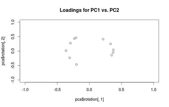
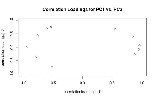
To clear up the terminological confusion: what the R package calls "loadings" are principal axes, and what it calls "correlation loadings" are (for PCA done on the correlation matrix) in fact loadings. As you noticed yourself, they differ only in scaling. What is better to plot, depends on what you want to see. Consider a following simple example:

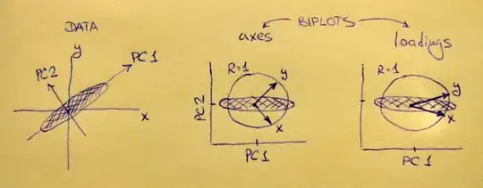
Left subplot shows a standardized 2D dataset (each variable has unit variance), stretched along the main diagonal. Middle subplot is a biplot: it is a scatter plot of PC1 vs PC2 (in this case simply the dataset rotated by 45 degrees) with rows of $\mathbf{V}$ plotted on top as vectors. Note that $x$ and $y$ vectors are 90 degrees apart; they tell you how the original axes are oriented. Right subplot is the same biplot, but now vectors show rows of $\mathbf{L}$. Note that now $x$ and $y$ vectors have an acute angle between them; they tell you how much original variables are correlated with PCs, and both $x$ and $y$ are much stronger correlated with PC1 than with PC2. I guess that most people most often prefer to see the right type of biplot.

Note that in both cases both $x$ and $y$ vectors have unit length. This happened only because the dataset was 2D to start with; in case when there are more variables, individual vectors can have length less than $1$, but they can never reach outside of the unit circle. Proof of this fact I leave as an exercise.

Let us now take another look at the mtcars dataset. Here is a biplot of the PCA done on correlation matrix:

Black lines are plotted using $\mathbf{V}$, red lines are plotted using $\mathbf{L}$.

And here is a biplot of the PCA done on the covariance matrix:

Here I scaled all the vectors and the unit circle by $100$, because otherwise it would not be visible (it is a commonly used trick). Again, black lines show rows of $\mathbf{V}$, and red lines show correlations between variables and PCs (which are not given by $\mathbf{L}$ anymore, see above). Note that only two black lines are visible; this is because two variables have very high variance and dominate the mtcars dataset. On the other hand, all red lines can be seen. Both representations convey some useful information.

P.S. There are many different variants of PCA biplots, see my answer here for some further explanations and an overview: Positioning the arrows on a PCA biplot. The prettiest biplot ever posted on CrossValidated can be found here.