It's best to think in terms of ratios, how much error is explained by $x$, how much is residual.
If we think of a super-simple regression with one independent variable and slope = 1, just $y = x + \epsilon$, then $\mathrm{Var}(Y) =\mathrm{Var}(X) + \mathrm{Var}(\epsilon)$. (Of course, using the assumption that the residual error $\epsilon$ is uncorrelated with $X$.) From that, it's straightforward that as the variance of $X$ increases, so does the variance of $Y$--if you observe a wider range of $X$ values, you'll also observe a wider range of $Y$ values.
However, we assume that the residual error is fixed, it doesn't change with $X$. And we know that R^2 is defined as the ratio of "explained variance" to "total variance". So
$$
R^2 = \frac{\mathrm{Var}(X)}{\mathrm{Var}(Y)} = \frac{\mathrm{Var}(X)}{\mathrm{Var}(X) + \mathrm{Var}(\epsilon)}
$$
And it's pretty clear that, given a fixed value of $\mathrm{Var}(\epsilon)$ as $\mathrm{Var}(X)$ increases the $R^2$ approaches 1.
This extends easily if the slope isn't equal to 1--the important assumption is that $\mathrm{Var}(X)$ and $\mathrm{Var}(\epsilon)$ are uncorrelated.
I find simulation a nice way to understand things too, you can see the effect with the following R code which simulates data for various values of $\mathrm{Var}(X)$ and $\mathrm{Var}(\epsilon)$, fits models, extracts the R squared values, and plots the results in a heatmap.
rsqd <- function(varx = 10, varresid = 3, n = 30, betax = 2) {
    x <- rnorm(n, sd = sqrt(varx))
    y <- betax * x + rnorm(n, sd = sqrt(varresid))
    return(summary(lm(y ~ x))$r.squared)
}

vx <- 1:20
vr <- 1:20

results <- expand.grid(vx = vx, vr = vr)
results$rsq <- numeric(nrow(results))

for (i in 1:nrow(results)) {
    results$rsq[i] <- rsqd(varx = results$vx[i], varresid = results$vr[i])
}

library(ggplot2)
ggplot(results, aes(x = vx, y = vr, fill = rsq)) + geom_tile()
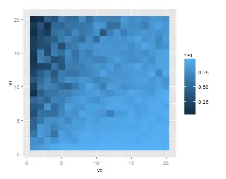
Despite the model always being "right", if the variation in x is small but the residual error is large, the R-squared is quite low (upper left corner). The situation is reversed in the lower right, where the residual error is small compared to the variation of x, and thus compared to the variation explained by x.