Why does my bootstrap interval have terrible coverage?

Question

I wanted to do a class demonstration where I compare a t-interval to a bootstrap interval and calculate the coverage probability of both. I wanted the data to come from a skewed distribution so I chose to generate the data as exp(rnorm(10, 0, 2)) + 1, a sample of size 10 from a shifted lognormal. I wrote a script to draw 1000 samples and, for each sample, calculate both a 95% t-interval and a 95% bootstrap percentile interval based on 1000 replicates.

When I run the script, both methods give very similar intervals and both have coverage probability of 50-60%. I was surprised because I thought the bootstrap interval would be better.

My question is, have I

• made a mistake in the code?
• made a mistake in calculating the intervals?
• made a mistake by expecting the bootstrap interval to have better coverage properties?

Also, is there a way to construct a more reliable CI in this situation?

 tCI.total <- 0
 bootCI.total <- 0
 m <- 10 # sample size
 true.mean <- exp(2) + 1

for (i in 1:1000){
 samp <- exp(rnorm(m,0,2)) + 1
 tCI <- mean(samp) + c(1,-1)*qt(0.025,df=9)*sd(samp)/sqrt(10)

 boot.means <- rep(0,1000)
 for (j in 1:1000) boot.means[j] <- mean(sample(samp,m,replace=T))
 bootCI <- sort(boot.means)[c(0.025*length(boot.means), 0.975*length(boot.means))]

 if (true.mean > min(tCI) & true.mean < max(tCI)) tCI.total <- tCI.total + 1
 if (true.mean > min(bootCI) & true.mean < max(bootCI)) bootCI.total <- bootCI.total + 1 
}
tCI.total/1000     # estimate of t interval coverage probability
bootCI.total/1000  # estimate of bootstrap interval coverage probability

Answer 1

Bootstrap diagnostics and remedies by Canto, Davison, Hinkley & Ventura (2006) seems to be a logical point of departure. They discuss multiple ways the bootstrap can break down and - more importantly here - offer diagnostics and possible remedies:

1. Outliers
2. Incorrect resampling model
3. Nonpivotality
4. Inconsistency of the bootstrap method

I don't see a problem with 1, 2 and 4 in this situation. Let's look at 3. As @Ben Ogorek notes (although I agree with @Glen_b that the normality discussion may be a red herring), the validity of the bootstrap depends on the pivotality of the statistic we are interested in.

Section 4 in Canty et al. suggests resampling-within-resamples to get a measure of bias and variance for the parameter estimate within each bootstrap resample. Here is code to replicate the formulas from p. 15 of the article:

library(boot)
m <- 10 # sample size
n.boot <- 1000
inner.boot <- 1000

set.seed(1)
samp.mean <- bias <- vars <- rep(NA,n.boot)
for ( ii in 1:n.boot ) {
    samp <- exp(rnorm(m,0,2)) + 1
    samp.mean[ii] <- mean(samp)
    foo <- boot(samp,statistic=function(xx,index)mean(xx[index]),R=inner.boot)
    bias[ii] <- mean(foo$t[,1])-foo$t0
    vars[ii] <- var(foo$t[,1])
}

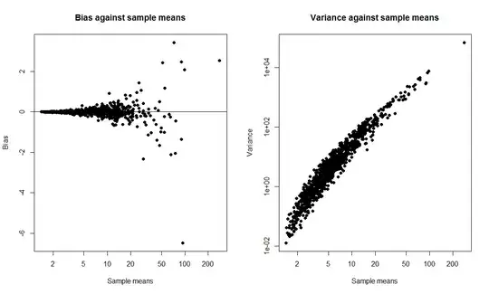
opar <- par(mfrow=c(1,2))
    plot(samp.mean,bias,xlab="Sample means",ylab="Bias",
        main="Bias against sample means",pch=19,log="x")
    abline(h=0)
    plot(samp.mean,vars,xlab="Sample means",ylab="Variance",
        main="Variance against sample means",pch=19,log="xy")
par(opar)

Note the log scales - without logs, this is even more blatant. We see nicely how the variance of the bootstrap mean estimate goes up with the mean of the bootstrap sample. This to me looks like enough of a smoking gun to attach blame to nonpivotality as a culprit for the low confidence interval coverage.

However, I'll happily admit that one could follow up in lots of ways. For instance, we could look at how whether the confidence interval from a specific bootstrap replicate includes the true mean depends on the mean of the particular replicate.

As for remedies, Canty et al. discuss transformations, and logarithms come to mind here (e.g., bootstrap and build confidence intervals not for the mean, but for the mean of the logged data), but I couldn't really make it work.

Canty et al. continue to discuss how one can reduce both the number of inner bootstraps and the remaining noise by importance sampling and smoothing as well as add confidence bands to the pivot plots.

This might be a fun thesis project for a smart student. I'd appreciate any pointers to where I went wrong, as well as to any other literature. And I'll take the liberty of adding the diagnostic tag to this question.

Answer 2

While I agree with Stephan Kolassa's analysis and conclusion, $$\hat{\mu} - \mu$$ with $\hat{\mu}$ the sample mean is definitely not an approximate pivot, let me make an additional remark. I investigated the use of the $t$-statistic $$\sqrt{m} \frac{\hat{\mu} - \mu}{\hat{\sigma}}$$ together with bootstrapping. The result was a coverage of around 0.8. Not a complete solution, but an improvement.

Then I thought a little more about the whole setup. With only 10 observations and an extremely skewed distribution, is it then not basically impossible to nonparametrically estimate the mean let alone construct confidence intervals with the right coverage?

The log-normal distribution considered has mean $e^2 + 1 = 8.39$. Since $P(X \leq 2) = 0.84$ when $X \sim \mathcal{N}(0,4)$ the mean is the $0.84$-quantile of the distribution! It means that the probability that all 10 observations are smaller than the mean is $0.84^{10} = 0.178$. So in a little less than 18% of the cases, the largest observation is smaller than the mean. To get a coverage greater than 0.82 we need a construction of a confidence interval for the mean the extends beyond the largest observation. I have a hard time imagining how such a construction can be made (and justified) without prior assumptions that the distribution is extremely skewed. But I welcome any suggestions.

Answer 3

The calculations were right, I cross-checked with the well-known package boot. Additionally I added the BCa-interval (by Efron), a bias-corrected version of the percentile bootstrap interval:

for (i in 1:1000) {
  samp <- exp(rnorm(m, 0, 2)) + 1

  boot.out <- boot(samp, function(d, i) sum(d[i]) / m, R=999)
  ci <- boot.ci(boot.out, 0.95, type="all")

  ##tCI <- mean(samp) + c(1,-1)*qt(0.025,df=9)*sd(samp)/sqrt(10)
  tCI <- ci$normal[2:3]
      percCI <- ci$perc[4:5]
  bcaCI <- ci$bca[4:5]
      boottCI <- ci$student[4:5]

  if (true.mean > min(tCI) && true.mean < max(tCI)) tCI.total <- tCI.total + 1
  if (true.mean > min(percCI) && true.mean < max(percCI)) percCI.total <- percCI.total + 1 
  if (true.mean > min(bcaCI) && true.mean < max(bcaCI)) bcaCI.total <- bcaCI.total + 1
}

tCI.total/1000     # estimate of t interval coverage probability
0.53
percCI.total/1000  # estimate of percentile interval coverage probability
0.55
bcaCI.total/1000  # estimate of BCa interval coverage probability
0.61

I assume the intervals would be far better if the original sample size is larger then 10, say 20 or 50.

Furthermore the bootstrap-t method usually leads to better results for skewed statistics. However it needs a nested loop and therefore 20+ times more computational time.

For hypothesis testing it is also very important that the 1-sided coverages are good. So looking only at the 2-sided coverages can often be misleading.

Answer 4

I was confused about this too, and I spent a lot of time of on the 1996 DiCiccio and Efron paper Bootstrap Confidence Intervals, without much to show for it.

It actually led me to think less of the bootstrap as a general purpose method. I used to think of it as something that would pull you out of a jam when you were really stuck. But I've learned its dirty little secret: bootstrap confidence intervals are all based on normality in some way or another. Allow me to explain.

The bootstrap gives you an estimate of the sampling distribution of the estimator, which is all you could ever hope for, right? But recall that the classical link between the sampling distribution and the confidence interval is based on finding a pivotal quantity. For anyone who's rusty, consider the case where $$x \sim N(\mu, \sigma^2)$$ and $\sigma$ is known. Then the quantity $$z = \frac{x - \mu}{\sigma} \sim N(0,1)$$ is pivotal, i.e., its distribution doesn't depend on $\mu$. Therefore, $\Pr(-1.96 \le \frac{x - \mu}{\sigma} \le 1.96) = 0.95$ and the rest is history.

When you think about what justifies the percentiles of the normal distribution being related to confidence intervals, it is entirely based on this convenient pivotal quantity. For an arbitrary distribution, there is no theoretical link between the percentiles of the sampling distribution and confidence intervals, and taking raw proportions of the bootstrap sampling distribution doesn't cut it.

So Efron's BCa (bias corrected) intervals use transformations to get to approximate normality and bootstrap-t methods rely on the resulting t-statistics being approximately pivotal. Now the bootstrap can estimate the hell out of moments, and you can always assume normality and use the standard +/-2*SE. But considering all the work that went into going non-parametric with the bootstrap, it doesn't seem quite fair, does it?

Answer 5

Check out Tim Hesterberg's article in The American Statistician at http://www.timhesterberg.net/bootstrap#TOC-What-Teachers-Should-Know-about-the-Bootstrap:-Resampling-in-the-Undergraduate-Statistics-Curriculum.

Essentially, the bootstrap percentile interval does not have strong coverage probability for skewed data unless n is large.