Pitfalls to avoid when transforming data?

Question

I achieved a strong linear relationship between my $X$ and $Y$ variable after doubly transforming the response. The model was $Y\sim X$ but I transformed it to $\sqrt{\frac{Y}{X}}\sim \sqrt{X}$ improving $R^2$ from .19 to .76.

Clearly I did some decent surgery on this relationship. Can anyone discuss the pitfalls of doing this, such as dangers of excessive transformations or possible violations of statistical principles?

From what you have, from the algebra alone it looks like just $Y \propto X^2$. Can you post the data or show a graph? Are there scientific reasons to expect $Y = 0$ when $X = 0$? — Nick Cox, Mar 16 '14 at 10:10
@NickCox: I think $Y\sim X$ is unconventional notation for $\mathrm{E} Y=\beta_0 + \beta_1 X$; perhaps the OP is speaking R rather than maths (something to be discouraged of course). — Scortchi - Reinstate Monica, Mar 16 '14 at 19:12
@Scortchi I fear you're right. Seeing the data would help either way. — Nick Cox, Mar 16 '14 at 20:00
In this case a 0 X would imply a 0 Y as Y is driving deaths and X is total KM's driven by all drivers. — Info5ek, Mar 16 '14 at 20:28
Have you considered a power function $Y = \alpha X^\beta$ often estimated by regression of $\log Y$ on $\log X$? — Nick Cox, Mar 16 '14 at 23:53
You have X on both sides. Of course X's root will predict the root of an otherwise random variable with X in the denominator. This is quite useless I would think. — Aaron Hall, Mar 17 '14 at 00:06
@AaronHall The equation isn't *necessarily* useless, since (multiplying back by $\sqrt X$ it's $\sqrt Y = \beta_0 \sqrt X + \beta_1 X + \sqrt X\epsilon$, which may well be a potentially plausible model in some situations). However the $R^2$ on the form of the equation given in the question isn't much use you can't compare it with something fitted on a different scale. (Incidentally, if that was your downvote on my answer, an explanation of what you think is wrong in the answer would be useful.) — Glen_b, Mar 17 '14 at 02:22

Glen_b · Accepted Answer · 2014-03-17T03:48:28.297

You can't really compare $R^2$ before and after, because the underlying variability in $Y$ is different. So you literally can take no comfort whatever from the change in $R^2$. That tells you nothing of value in comparing the two models.

The two models are different in several ways, so they mean different things -- they assume very different things about the shape of the relationship and the variability of the error term (when considered in terms of the relationship between $Y$ and $X$). So if you're interested in modelling $Y$ (if $Y$ itself is meaningful), produce a good model for that. If you're interested in modelling $\sqrt Y$ (/$\sqrt Y$ is meaningful), produce a good model for that. If $\sqrt{Y/X}$ carries meaning, then make a good model for that. But compare any competing models on comparable scales. $R^2$ on different responses simply aren't comparable.

If you're just trying different relationships in the hope of finding a transformation with a high $R^2$ -- or any other measure of 'good fit' -- the properties of any inference you might like to conduct will be impacted by the existence of that search process.

Estimates will tend to be biased away from zero, standard errors will be too small, p-values will be too small, confidence intervals too narrow. Your models will on average appear to be 'too good' (in the sense that their out-of-sample behavior will be disappointing compared to in-sample behavior).

To avoid this kind of overfitting, you need, if possible, to do the model-identification and estimation on different subsets of the data (and model evaluation on a third). If you repeat this kind of procedure on many "splits" of the data taken at random, you get a better sense of how reproducible your results are.

There are many posts here with relevant points on these issues: it might be worth trying some searches.

(If you have good a priori reasons for choosing a particular transformation, that's a different issue. But searching the space of transformations to find something that fits carries all manner of 'data snooping' type problems with it.)

Thanks for the response Glen. The reason I did this transformation is because its the only one that didn't give me biased residuals. I tried the standard y/x, log(y), sqrt(y) and various combinations of those. All resulted in a sloping residual plot. Only after doing a two stage transformation did I get random appearing residuals. However you state that this model is potentially uninformative for out-of-sample data as I may have just overfit the data, correct? — Info5ek, Mar 16 '14 at 00:43
Well, yes, but it's a problem with any form of model-specification when looking at the data, so it happens a lot. In many situations it's hard to avoid, which is where the sample-splitting can come in. (Cross-validation can be a handy tool for such situations.) — Glen_b, Mar 16 '14 at 00:47
It would be useful to know the reasons for the downvote. What's wrong with the answer? Perhaps it can be improved. (If it can't be improved, why the downvote?) — Glen_b, Mar 17 '14 at 02:17
@Glen_b: Tricky to cross-validate an ill-defined procedure though - in each fold you'd need to repeat the process of looking at diagnostics, thinking up another transformation when you didn't like them, trying that, & so on. — Scortchi - Reinstate Monica, Mar 19 '14 at 10:14
@Scortchi Yes, if the transformations aren't being selected from a known pool of candidates by some simple rule, it may be impossible. — Glen_b, Mar 19 '14 at 20:23

score 16 · Answer 2 · edited Mar 16 '14 at 10:13

16

There's a bigger problem than the ones identified by @Glen_b .

set.seed(123)
x <- rnorm(100, 20, 2)
y <- rnorm(100, 20, 2)
dv <- (y/x)^.5
iv <- x^.5
m1 <- lm(dv~iv)
summary(m1)

And I get an $R^2$ of 0.49 and a P-value that is $5.5 \times 10^{-16}$.

You have $X$ on both sides of the equation.

edited Mar 16 '14 at 10:13

Nick Cox

48,377
8
110
156

answered Mar 16 '14 at 01:02

Peter Flom

94,055
35
143
276

2

Not sure that's a different problem to not having good a priori reasons to express the model one way rather than another. If you let $W=\sqrt{\frac{Y}{X}}$ & $Z=\sqrt{X}$ then you can just as well say that the first model ($Y\sim X$) has $Z^2$ on both sides of the equation. – Scortchi - Reinstate Monica Mar 16 '14 at 01:17
But if X and Y are random noise then you get a strong relationship in my example. Do you in your version with X and Y? No. – Peter Flom Mar 16 '14 at 09:10
@PeterFlom is correct, this is spurious correlation. See for example [Kenney, 1982](http://onlinelibrary.wiley.com/doi/10.1029/WR018i004p01041/abstract) – Tony Ladson Mar 16 '14 at 11:56
4

If $W$ & $Z$ are random noise, regressing $Y$ on $X$ gives a strong relationship. Whence the asymmetry that labels one regression spurious rather than the other without consideration of what the variables even mean? This kind of thing was debated between Pearson & Yule ([Aldrich (1995)](https://projecteuclid.org/euclid.ss/1177009870)) & I'm with Yule: what's spurious isn't the correlation but the claim of a causal relationship based on that correlation. – Scortchi - Reinstate Monica Mar 16 '14 at 12:23
1

Yeah, but here, the regression started with X and Y. Doesn't it matter which variables are, so to speak, *the* variables? – Peter Flom Mar 16 '14 at 13:36
2

Can't see why it should, except insofar as, as @Glen_b points out in his first sentence, if your goal was to predict $Y$, then a high coefficient of determination of a model for $W$ is nothing to crow about. And of course if you have strong ideas about what the error term looks like, one model is more tractable than the other. – Scortchi - Reinstate Monica Mar 16 '14 at 19:06
If your a priori model is that $\sqrt{\frac{Y}{X}}\sim \sqrt{X}$ then it seems to me that you can't use regresion to test it, as that relationship exists even if there is nothing but noise in both variables – Peter Flom Mar 16 '14 at 20:39
4

You raise a good point about W & Z, @Scortchi, but it seems to me that it matters what you consider the variables you care about are, & what variables you created just to get a better model. Which are the real variables is determined by the meaning of X etc, in the context of the substantive question. I infer from the text that the OP wants to understand the relationship b/t X & Y, & created W & Z to improve the model fit. Ie, in this concrete case, it seems to me that Peter is right, you can't try to improve your model by putting X on both sides. – gung - Reinstate Monica Mar 16 '14 at 21:56
1

@gung "*it matters what you consider the variables you care about are*" -- I believe that point has been made by both Scortchi and myself here already. Certainly Scortchi made it explicit in his comments, even if it wasn't completely obvious in mine. – Glen_b Mar 17 '14 at 03:45
I agree w/ you, @Glen_b. I was trying to state that the point was a good 1 & had been made, & there was nothing left to argue about, since (as Peter noted) X & Y were the variables the OP cares about. I don't know who the downvoter was, but it wasn't me. – gung - Reinstate Monica Mar 17 '14 at 04:12
@gung Okay, sorry I misunderstood. (I *didn't* think it was your downvote, not that it's important -- I just like to know what the problem is when I get one; usually there's something that can be improved.) – Glen_b Mar 17 '14 at 04:36
Then perhaps the whole "debate" is a misunderstanding? (That often happens) – Peter Flom Mar 17 '14 at 10:04
@gung: My point's that, after the two (bad enough) problems identified by Glen_b in the way the $w_i=\beta_0 + \beta_1 z_i +\epsilon_i$ model was conjured up, I don't believe there's a third problem arising from one way of expressing its mathematical form. If you rewrite it to have $y$ as the response it's a *different* model from $y_i=\beta_0 + \beta_1 x_i +\varepsilon_i$; like any other model it can be criticised for being incompatible with substantive knowledge or for not fitting the data, or aspersions can be cast on its pedigree (as in this case): but it doesn't suffer from some – Scortchi - Reinstate Monica Mar 17 '14 at 10:12
1

inherent spuriousness or infidelity to the "true" variables. Peter's example is instructive in the same way that Simpson's paradox is instructive, but can't justify ruling out certain models *tout court.* The lessons to be drawn from it are these: (1) Model mis-specification is not always apparent (look at the diagnostic plots from `m1`). (2) Mis-specified models can still have predictive value ("spurious" correlation is correlation nonetheless). (3) Correlation $\neq$ causation. – Scortchi - Reinstate Monica Mar 17 '14 at 10:13
Perhaps we should take this to chat? – Peter Flom Mar 17 '14 at 10:15
1

IMHO this answer takes the discussion in the wrong direction because it can mislead in several ways: (a) there is no problem creating models having "$x$" on both sides when that is indicated by theory or exploratory analysis; (b) although the code *starts* with independent variables $x$ and $y$, it *creates* interdependent variables $iv$ and $dv$ (whence there is no surprise at finding a "significant" result) but (c) OLS regression is inappropriate for these variables. As such it sheds no light on the key issue (of selecting transformations in models) and its conclusion is less than helpful. – whuber Mar 17 '14 at 15:12
@Peter: Sorry I didn't go into chat, but I thought that even if it turns out we don't really disagree on anything fundamental (quite likely), others might still draw the wrong conclusions from your example so I'd rather go into more detail about it in an answer. And if there's a flaw in my reasoning, the more people looking, the more likely someone is to spot it. – Scortchi - Reinstate Monica Mar 18 '14 at 12:29

Scortchi - Reinstate Monica · Answer 3 · 2014-03-19T19:16:41.270

There are two elements to @Peter's example, which it might be useful to disentangle:

(1) Model mis-specification. The models

$$y_i = \beta_0 + \beta_1 x_i + \varepsilon_i \qquad\text{(1)}$$

&

$$w_i=\gamma_0 + \gamma_1 z_i + \zeta_i \qquad\text{(2)}$$

, where $w_i=\sqrt{\frac{y_i}{x_i}}$ & $z_i=\sqrt{x_i}$, can't both be true. If you re-express each in terms of the other's response they become non-linear in the parameters, with heteroskedastic errors.

$$w_i = \sqrt{\frac{\beta_0}{z_i^2} + \beta_1 + \frac{\varepsilon_i}{z_i^2}} \qquad\text{(1)}$$

$$y_i = (\gamma_0 \sqrt x_i + \gamma_1 \sqrt x_i + \zeta_i \sqrt x_i)^2 \qquad\text{(2)}$$

If $Y$ is assumed to be a Gaussian random variable independent of $X$, then that's a special case of Model 1 in which $\beta_1=0$, & you shouldn't be using Model 2. But equally if $W$ is assumed to be a Gaussian random variable independent of $Z$, you shouldn't be using Model 1. Any preference for one model rather than the other has to come from substantive theory or their fit to data.

(2) Transformation of the response. If you knew $Y$ & $X$ to be independent Gaussian random variables, why should the relation between $W$ & $Z$ still surprise you, or would you call it spurious? The conditional expectation of $W$ can be approximated with the delta method:

$$ \operatorname{E} \sqrt\frac{Y}{x} = \frac{\operatorname{E}\sqrt{Y}}{z} \\ \approx \frac{\sqrt{\beta_0} + \frac{\operatorname{Var}{Y}}{8\beta_0^{3/2}}}{z}$$

It is indeed a function of $z$.

Following through the example ...

set.seed(123)
x <- rnorm(100, 20, 2)
y <- rnorm(100, 20, 2)
w <- (y/x)^.5
z <- x^.5
wrong.model <- lm(w~z)
right.model <- lm(y~x)
x.vals <- as.data.frame(seq(15,25,by=.1))
names(x.vals) <- "x"
z.vals <- as.data.frame(x.vals^.5)
names(z.vals) <- "z"
plot(x,y)
lines(x.vals$x, predict(right.model, newdata=x.vals), lty=3)
lines(x.vals$x, (predict(wrong.model, newdata=z.vals)*z.vals)^2, lty=2)
abline(h=20)
legend("topright",legend=c("data","y on x fits","w on z fits", "truth"), lty=c(NA,3,2,1), pch=c(1,NA,NA,NA))
plot(z,w)
lines(z.vals$z,sqrt(predict(right.model, newdata=x.vals))/as.matrix(z.vals), lty=3)
lines(z.vals$z,predict(wrong.model, newdata=z.vals), lty=2)
lines(z.vals$z,(sqrt(20) + 2/(8*20^(3/2)))/z.vals$z)
legend("topright",legend=c("data","y on x fits","w on z fits","truth"),lty=c(NA,3,2,1), pch=c(1,NA,NA,NA))

enter image description here

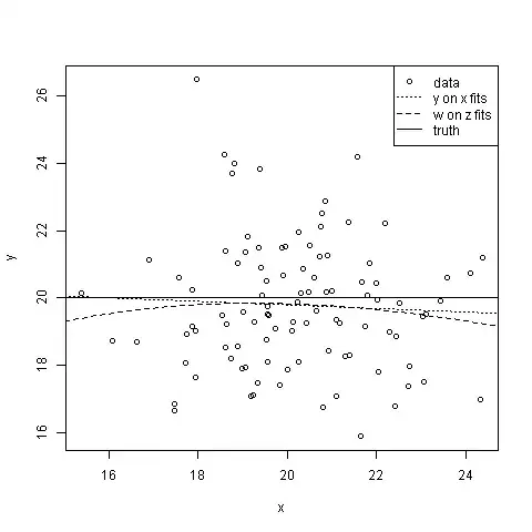
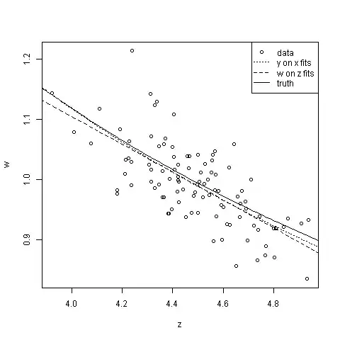
Neither Model 1 nor Model 2 is much use for predicting $y$ from $x$, but both are all right for predicting $w$ from $z$: mis-specification hasn't done much harm here (which isn't to say it never will—when it does, it ought to be apparent from the model diagnostics). Model-2-ers will run into trouble sooner as they extrapolate further away from the data—par for the course, if your model's wrong. Some will gain pleasure from contemplation of the little stars they get to put next to their p-values, while some Model-1-ers will bitterly grudge them this—the sum total of human happiness stays about the same. And of course, Model-2-ers, looking at the plot of $w$ against $z$, might be tempted to think that intervening to increase $z$ will reduce $w$—we can only hope & pray they don't succumb to a temptation we've all been incessantly warned against; that of confusing correlation with causation.

Aldrich (2005), "Correlations Genuine and Spurious in Pearson and Yule", Statistical Science, 10, 4 provides an interesting historical perspective on these issues.

score 3 · Answer 4 · answered Mar 18 '14 at 12:22

The earlier answer of @Glen_b is all important. Playing with transformations distorts every part of statistical inference and results in $R^2$ that is biased high. In short, not having a parameter in the model for everything you don't know will give a false sense of precision. That's why regression splines are now so popular.

Pitfalls to avoid when transforming data?

4 Answers4

Linked