Marginal effect of squared variable in Probit Model

Question

I want to estimate the following probit model

$employed_t=\beta_1 age + \beta_2 age^2$

and I use the Stata code

probit employed c.age##c.age

Using the command margins I obtain the marginal effect of $age$ including the effect through the quadratic terms if included in the model (see: How do I interpret a probit model in Stata?).

How do I obtain the marginal effect for the quadratic terms $age^2$?

Is this procedure correct?

probit employed c.age##c.age

sum age

local m=r(mean)

local x1 _b[c.age]*'m'+_b[c.age#c.age]*'m'+_b[_cons]

nlcom 2*normd('x1')*_b[c.age#c.age]-('x1')*normd('x1')*(_b[c.age]+2*_b[c.age#c.age]*'r')

Answer 1

I am inclined to agree with @StasK's comment. However, something like what you want is feasible, though a little tricky to interpret. What I propose below tells you how the marginal effect of $x$ varies with $x$.

You know that the conditional mean of the dependent variable in a probit model is $$\mathbb{Pr}[y=1 \vert x,z]=\Phi(\alpha + \beta \cdot x + \gamma \cdot x^2+z'\pi).$$ The variable $x$ is what we care about. The vector $z$ contains some other covariates. $\Phi(.)$ is the standard normal cdf, and $\varphi(.)$ is is the standard normal pdf, which will be used below.

The marginal effect of $x$ is $$\frac{\partial \mathbb{Pr}[y=1 \vert x,z]}{\partial x}=\varphi(\alpha + \beta \cdot x + \gamma \cdot x^2+z'\pi)\cdot(\beta + 2\cdot\gamma \cdot x).$$ The change in the marginal effect is the second derivative $$ \frac{\partial^2 \mathbb{Pr}[y=1 \vert x,z]}{\partial x^2} = \varphi(\alpha + \beta \cdot x + \gamma \cdot x^2+z'\pi)\cdot(2\cdot\gamma) +(\beta + 2\cdot\gamma \cdot x)\cdot\varphi'(\alpha + \beta \cdot x + \gamma \cdot x^2+z'\pi). $$

Since $\varphi′(x)=−x \cdot \varphi(x)$, this "simplifies" to

$$ \frac{\partial^2 \mathbb{Pr}[y=1 \vert x,z]}{\partial x^2} = \varphi(\alpha + \beta \cdot x + \gamma \cdot x^2+z'\pi)\cdot \left[ 2\cdot\gamma -(\beta + 2\cdot\gamma \cdot x)^2\cdot(\alpha + \beta \cdot x + \gamma \cdot x^2+z'\pi)\right]. $$

Note that this is a function of $x$ and $z$s, so we can evaluate this quantity at various possible values. Also note that while the first term is surely positive since it is a normal density, it's hard to sign the second term even if you know the sign and magnitude of the coefficients.

Assuming that I didn't screw up the derivative, here's how I might actually do this in Stata:

#delimit;
sysuse auto, clear;
probit foreign c.mpg##c.mpg c.weight, coefl;
/* At own values of covarites */
margins, expression(normalden(predict(xb))*(2*_b[c.mpg#c.mpg] - predict(xb)*(_b[c.mpg]+2*_b[c.mpg#c.mpg]*mpg)^2));
/* At chosen values of covarites */
margins, expression(normalden(predict(xb))*(2*_b[c.mpg#c.mpg] - predict(xb)*(_b[c.mpg]+2*_b[c.mpg#c.mpg]*mpg)^2)) at(mpg=20 weight=3000);
/* At avermpg value of covariates */
margins, expression(normalden(predict(xb))*(2*_b[c.mpg#c.mpg] - predict(xb)*(_b[c.mpg]+2*_b[c.mpg#c.mpg]*mpg)^2)) atmeans;

If I was doing this myself and feeling lazy, I might use adjacent reverse contrasts. For instance, here's the second derivative evaluated at 4 values of $x$:

margins, expression(normalden(predict(xb))*(2*_b[c.mpg#c.mpg] - predict(xb)*(_b[c.mpg]+2*_b[c.mpg#c.mpg]*mpg)^2)) at(mpg = (10 20 30 40));

Here's a comparison of the derivatives. This compares the marginal effects of mpg at mpg of x+1 to the marginal effect at mpg of x:

margins, dydx(mpg) at(mpg = (10 11 20 21 30 31 40 41)) contrast(atcontrast(ar(2(2)8)._at) wald);

Note how close the two commands' outputs are, but the second is so much easier.

I don't know what r is your code, so I can't verify if what you have is correct.

Answer 2

I don't use stata for GLMs (like probit), so maybe I'm missing something specific to the context, but anyway:

What you're doing is modeling $$ g(E[employed]) = \beta_0 + \beta_1age + \beta_2age^2 $$ where $g(.)$ is the normal cdf. You can follow the following procedure to interpret your coeffcients (which is almost exactly the same for logit):

1. Draw or graph for yourself the normal cdf. It is sigmoidal.
2. Note the intercept ($\beta_0$) on your x-axis, and draw a line up to where it intersects the normal cdf.
3. For a given age $A$, move $\beta_1 A + \beta_2 A^2$ from your intercept. Note the point on the x-axis, and draw a line up to where it intersects the function.
4. Draw a line to the left, to see where it intersects the y-axis. This is a probability.
5. Voila: you've got the fitted value of $\widehat{employed}$ for a given level of age. Over a gradient of values of $A$, you get a quadratic marginal effect curve.

Answer 3

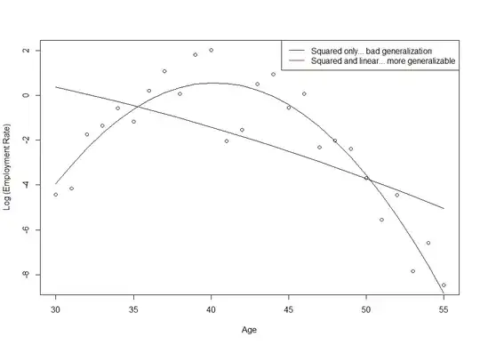
If you don't adjust for $\mbox{age}$ in this model when including $\mbox{age}^2$ as a regressor, you are forcing the instantaneous rate of employment decrease to be zero at $\mbox{age}=0$. That might seem contrived, but if you take a change of variable:

$$\mbox{age}^* = \frac{\mbox{age} - 50}{5}$$

You might see why that would be a stupid idea. You can prove that any data with a strong non-zero linear term in a quadratic mean model will look locally consistent with a reduced model dropping the linear term. So don't let the data decide which terms to use. Use them both as a form of "added assurance" or "added insurance".