Binary classification using radial basis kernel SVM with a single feature

Question

Is there any interpretation (graphical or otherwise) of a radial basis kernel SVM being trained with a single feature? I can visualize the effect in 2 dimensions (the result being a separation boundary that is curved rather than a linear line. (e.g http://en.wikipedia.org/wiki/File:Kernel_Machine.png).

I'm having trouble thinking of what this would be like if your original data only had a single feature. What would the boundary line look like for this case?

score 4 · Accepted Answer · answered Feb 13 '14 at 17:22

You can play with this code: (taken and modify from: http://scikit-learn.org/stable/auto_examples/svm/plot_iris.html)

I cheated a bit to have only one feature but I guess you get the point. Just think of it in 2D using only a line and not in 3D

import numpy as np
import pylab as pl
from sklearn import svm, datasets


def linearly_separable_data():
    X = np.r_[ np.random.randn(20,2) - [3,3], np.random.randn(20,2) + [4,4]] 
    X[:,1] = 0 
    Y = [0]*20 + [1]*20 
    return X, Y


def non_linearly_separable_data():
    X = np.r_[ np.random.randn(20,2) - [3,3], np.random.randn(20,2) + [2,2], np.random.randn(20,2) + [5,5]] 
    X[:,1] = 0 
    Y = [0]*20 + [1]*20 + [0]*20  
    return X, Y


X, Y = non_linearly_separable_data()
h = .02  # step size in the mesh

# we create an instance of SVM and fit out data. We do not scale our
# data since we want to plot the support vectors
C = 1.0  # SVM regularization parameter
svc = svm.SVC(kernel='linear', C=C).fit(X, Y)
rbf_svc = svm.SVC(kernel='rbf', gamma=0.7, C=C).fit(X, Y)
poly_svc = svm.SVC(kernel='poly', degree=3, C=C).fit(X, Y)
lin_svc = svm.LinearSVC(C=C).fit(X, Y)

# create a mesh to plot in
x_min, x_max = X[:, 0].min() - 1, X[:, 0].max() + 1
y_min, y_max = X[:, 1].min() - 1, X[:, 1].max() + 1
xx, yy = np.meshgrid(np.arange(x_min, x_max, h),
                     np.arange(y_min, y_max, h))

# title for the plots
titles = ['SVC with linear kernel',
          'SVC with RBF kernel',
          'SVC with polynomial (degree 3) kernel',
          'LinearSVC (linear kernel)']


for i, clf in enumerate((svc, rbf_svc, poly_svc, lin_svc)):
    # Plot the decision boundary. For that, we will assign a color to each
    # point in the mesh [x_min, m_max]x[y_min, y_max].
    pl.subplot(2, 2, i + 1)
    Z = clf.predict(np.c_[xx.ravel(), yy.ravel()])
    # Put the result into a color plot
    Z = Z.reshape(xx.shape)
    pl.contourf(xx, yy, Z, cmap=pl.cm.Paired)
    pl.axis('off')
    # Plot also the training points
    pl.scatter(X[:, 0], X[:, 1], c=Y, cmap=pl.cm.Paired)
    pl.title(titles[i])

pl.show()

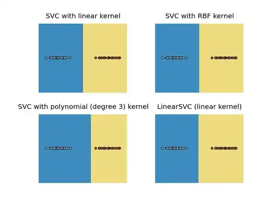
For linearly separable:

Linearly separable

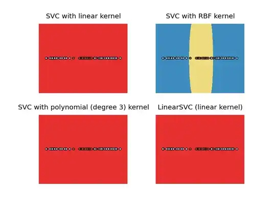
And for non-linearly separable:

Non-Linearly separable

So for the linearly separable case, you got a point separating the two classes. And for non-linearly separable, you got an interval.

Binary classification using radial basis kernel SVM with a single feature

1 Answers1