6

I am using the parametric approach and non-parametric (local linear regression) approaches of regression discontinuity design (RDD) to compute the treatment effect using Stata.

To get the user-written rd and the 102nd Congress data, I do this:

net get rd
use votex

The local linear approach:

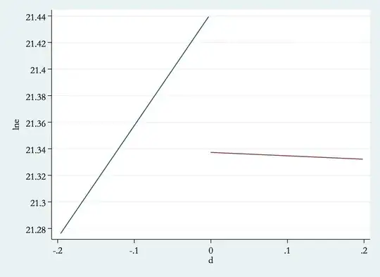
rd lne d,bw(0.20) mbw(100) ker(rec)
Two variables specified; treatment is 
assumed to jump from zero to one at Z=0. 

 Assignment variable Z is d
 Treatment variable X_T unspecified
 Outcome variable y is lne

Estimating for bandwidth .2
------------------------------------------------------------------------------
         lne |      Coef.   Std. Err.      z    P>|z|     [95% Conf. Interval]
-------------+----------------------------------------------------------------
       lwald |  -.1046939   .1147029    -0.91   0.361    -.3295075    .1201197
-----------------------------------------------------------------------------

As far as I understand this is equivalent to following :

gen win_d=win*d
reg lne d win win_d if d>=-0.2 & d<=0.2

      Source |       SS       df       MS              Number of obs =     267
-------------+------------------------------           F(  3,   263) =    0.43
       Model |  .271662326     3  .090554109           Prob > F      =  0.7339
    Residual |  55.7885045   263  .212123591           R-squared     =  0.0048
-------------+------------------------------           Adj R-squared = -0.0065
       Total |  56.0601668   266  .210752507           Root MSE      =  .46057

------------------------------------------------------------------------------
         lne |      Coef.   Std. Err.      t    P>|t|     [95% Conf. Interval]
-------------+----------------------------------------------------------------
           d |   .8450601   .7855123     1.08   0.283    -.7016333    2.391753
         win |  -.1046939   .1257913    -0.83   0.406    -.3523801    .1429923
       win_d |  -.8707605   1.048807    -0.83   0.407    -2.935887    1.194366
       _cons |   21.44195   .0925378   231.71   0.000     21.25974    21.62415
------------------------------------------------------------------------------

However, when we use the parametric approach (let's say with the polynomial of order one), we use all the observations. But, I am trying to see how parametric approach can be compared with non-parametric approach with the same number of observation as in non-parametric approach. So, I do as follows:

reg lne d win if d>=-0.2 & d<=0.2

      Source |       SS       df       MS              Number of obs =     267
-------------+------------------------------           F(  2,   264) =    0.30
       Model |  .125446108     2  .062723054           Prob > F      =  0.7440
    Residual |  55.9347207   264  .211873942           R-squared     =  0.0022
-------------+------------------------------           Adj R-squared = -0.0053
       Total |  56.0601668   266  .210752507           Root MSE      =   .4603

------------------------------------------------------------------------------
         lne |      Coef.   Std. Err.      t    P>|t|     [95% Conf. Interval]
-------------+----------------------------------------------------------------
           d |   .3566172   .5201877     0.69   0.494    -.6676274    1.380862
         win |  -.0964314   .1253232    -0.77   0.442    -.3431916    .1503288
       _cons |   21.39136   .0696112   307.30   0.000      21.2543    21.52843
------------------------------------------------------------------------------

My concern is why the non-parametric approach result (-.1046939) is not the same as parametric approach (-.0964314), although we are using the same observation for both.

dimitriy
  • 31,081
  • 5
  • 63
  • 138
user227710
  • 605
  • 7
  • 21

1 Answers1

5

This is happening because you are restricting the effect of Democratic vote share to be the same on both sides of the cutoff in your third specification, which is a slightly different model. As the magnitude and significance of the interaction term in (2) tells you, the slopes are actually somewhat different:

enter image description here

Graph code:

tw (lfit lne d if inrange(d,-.2,0)) (lfit lne d if inrange(d,0,.2)), legend(off) ylab(#15, angle(0)) ytitle("lne") xtitle("d")

You may want something like my third specification (though it it not clear what you have in mind with the comparison):

. use votex, clear
(102nd Congress)

. /* RD/local linear regression model */
. rd lne d, mbw(100) bw(0.2) ker(rec)
Two variables specified; treatment is 
assumed to jump from zero to one at Z=0. 

 Assignment variable Z is d
 Treatment variable X_T unspecified
 Outcome variable y is lne

Estimating for bandwidth .2
------------------------------------------------------------------------------
         lne |      Coef.   Std. Err.      z    P>|z|     [95% Conf. Interval]
-------------+----------------------------------------------------------------
       lwald |  -.1046939   .1147029    -0.91   0.361    -.3295075    .1201197
------------------------------------------------------------------------------

. 
. /* OLS Version With Interactions */
. reg lne c.d##i.win if d > -.2 & d < .2 // note that you can specify interaction on the fly

      Source |       SS       df       MS              Number of obs =     267
-------------+------------------------------           F(  3,   263) =    0.43
       Model |  .271662281     3  .090554094           Prob > F      =  0.7339
    Residual |  55.7885045   263  .212123591           R-squared     =  0.0048
-------------+------------------------------           Adj R-squared = -0.0065
       Total |  56.0601668   266  .210752507           Root MSE      =  .46057

------------------------------------------------------------------------------
         lne |      Coef.   Std. Err.      t    P>|t|     [95% Conf. Interval]
-------------+----------------------------------------------------------------
           d |     .84506   .7855123     1.08   0.283    -.7016333    2.391753
       1.win |  -.1046939   .1257913    -0.83   0.406    -.3523801    .1429923
             |
     win#c.d |
          1  |  -.8707604   1.048807    -0.83   0.407    -2.935887    1.194366
             |
       _cons |   21.44195   .0925378   231.71   0.000     21.25974    21.62415
------------------------------------------------------------------------------

. 
. /* OLS Model Without Interaction */
. reg lne d if d >= -.2 & d < 0 // fit a line to the left

      Source |       SS       df       MS              Number of obs =     109
-------------+------------------------------           F(  1,   107) =    1.58
       Model |  .245503732     1  .245503732           Prob > F      =  0.2116
    Residual |  16.6357215   107  .155474033           R-squared     =  0.0145
-------------+------------------------------           Adj R-squared =  0.0053
       Total |  16.8812252   108  .156307641           Root MSE      =   .3943

------------------------------------------------------------------------------
         lne |      Coef.   Std. Err.      t    P>|t|     [95% Conf. Interval]
-------------+----------------------------------------------------------------
           d |     .84506   .6724925     1.26   0.212    -.4880779    2.178198
       _cons |   21.44195   .0792234   270.65   0.000     21.28489      21.599
------------------------------------------------------------------------------

. reg lne d if d >= 0 & d < .2 // fit a line to the right

      Source |       SS       df       MS              Number of obs =     158
-------------+------------------------------           F(  1,   156) =    0.00
       Model |  .000290102     1  .000290102           Prob > F      =  0.9729
    Residual |   39.152783   156  .250979378           R-squared     =  0.0000
-------------+------------------------------           Adj R-squared = -0.0064
       Total |  39.1530731   157  .249382631           Root MSE      =  .50098

------------------------------------------------------------------------------
         lne |      Coef.   Std. Err.      t    P>|t|     [95% Conf. Interval]
-------------+----------------------------------------------------------------
           d |  -.0257003    .755932    -0.03   0.973    -1.518883    1.467483
       _cons |   21.33725   .0926828   230.22   0.000     21.15418    21.52033
------------------------------------------------------------------------------

. 
. di  "RD is "21.33725 - 21.44195 // TE is the diff in the intercepts 
RD is -.1047
dimitriy
  • 31,081
  • 5
  • 63
  • 138
  • Thank you very much for the explanation. In your `rd` command, I wonder whether degree (1) option is mandatory. I checked with different numbers (2,3,..10), but it give the same answer. – user227710 Feb 10 '14 at 15:28
  • 2
    Indeed. The degree option does not actually do anything. I'll take it out. `rd` always implements local linear regression. If you want higher order polynomials, try `rdrobust lne d, c(0) p(2) kernel(uniform) h(0.2)`. – dimitriy Feb 10 '14 at 18:07