This answer implements an approach along the lines of whuber's comment, where $p$ is estimated naively from the 10 tosses made at the start, and then 'plugged-in' to $P(F_{HH}|p)$ to get the prediction interval.
The approach does not explicitly account for uncertainty in $p$, which leads to poor performance in some cases, as shown below. If we had many more than 10 tosses available to estimate $p$, then this approach might work fine. It would be interesting to know of other approaches which can account for the uncertainty in $p$.
All code in this answer is in R.
Step 1: Code to compute $P(F_{HH}|p)$
Firstly, we need to be able to compute $P(F_{HH}|p)$. The following code does that analytically (since the simulation approach is very inefficient for small $p$):
pmf_FHH<-function(p, Nout){
#############################################################
#
# Analytically compute the probability mass function for F_HH
# F_HH = number of coin flips required to give 2 consecutive heads
#
#
# p = probability of heads (length 1 vector)
# Nout = integer vector of values for which we want the pmf
#

# Quick exit
if(p==0) return(Nout*0)
if(p==1) return((Nout==2))
if(max(Nout)==1) return(0*Nout)

# Recursively compute the pmf
N=max(Nout)

# Storage
PrN_T=rep(NA,N) # Probability that we got to the N'th flip without 2 consecutive heads, AND the N'th flip was a tail
PrN_2H=rep(NA,N) # Probability that the N'th flip gives 2 consecutive heads (for the first time)

# First flip
PrN_T[1]=(1-p) # Probability that we got to the first flip and it was a tail
PrN_2H[1]=0 # Can't have 2 heads on 1st flip

# Second flip
PrN_T[2] =(1- p) # Probability we get to the second flip and it was a tail
PrN_2H[2]=p*p # Probability that we get 2 heads after 2 flips

# Third flip and above
for(i in 3:length(PrN_2H)){
    # 'Probability that we got to the i'th flip, and it was a tail
    # = [1-(probability that we have terminated by i-1) ]*(1-p)
    PrN_T[i] = (1-sum(PrN_2H[1:(i-1)]))*(1-p)
    # Probability that flip i-2 was a tail, and i-1 and i were heads
    PrN_2H[i]=PrN_T[i-2]*p*p
}

return(PrN_2H[Nout])
}
To test the above function and for later use testing the prediction intervals, we write another function to simulate the coin toss process.
sim_FHH_p<-function(p,n=round(1e+04/p**3), pattern='11'){
# Simulate many coin toss sequences, ending in the first occurrence of pattern
#
# p = probability of 1 (1=heads)
# n = number of individual tosses to sample (split into sequences ending in pattern)
# pattern = pattern to split on (1=heads)
#
# returns vector with the length of each toss sequence

# Make a data string of many coin flips e.g. '011010011'.
random_data=paste(sample(c(0,1),n,replace=T,prob=c(1-p,p)),
                  collapse="")

# Split up by occurrence of pattern, count characters, and add the number of characters in pattern.
# Each element of random_FHH gives a number of coin-tosses to get pattern
random_FHH=nchar(unlist(strsplit(random_data,pattern)))+nchar(pattern)

# The last string may not have ended in pattern. Remove it.
random_FHH=random_FHH[-length(random_FHH)]

return(random_FHH)
}
Now I run a test to check that the simulated and analytical results are 'the same' (increase the 1e+07 to get better agreement).
set.seed(1)
p=0.3
# Simulate coin-toss
qq=sim_FHH_p(p,n=1e+07, pattern='11')

Nmax=round(10/p**2) # Convenient upper limit where we check pmf_FHH
empirical_pmf=rep(NA,Nmax)
for(i in 1:Nmax) empirical_pmf[i] = (sum(qq==i)/length(qq))

png('test_analytical_relation.png',width=6,height=5,res=200,units='in')
plot(1:Nmax,empirical_pmf,main='Test of analytical relation',ylab='pmf')
points(1:Nmax,pmf_FHH(p, 1:Nmax),col='red',t='l')
legend('topright', c('Approximate empirical pmf', 'Analytical pmf'), pch=c(1,NA),lty=c(NA,1),col=c(1,2))
dev.off()
It looks fine. 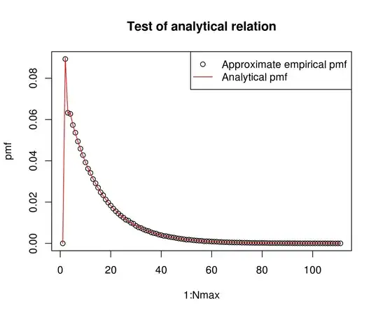
Step 2: Code to compute the prediction interval, assuming $p$ is known.
If p is known, then we can directly use $P(F_{HH}|p)$ to get a prediction interval for $F_{HH}$. For a one-sided (1-$\alpha$) prediction interval, we just need to get the (1-$\alpha$) quantile of $P(F_{HH}|p)$. The code is:
ci_FHH<-function(p, alpha=0.1,Nmax=round(10/max(p,0.001)**2), two.sided=FALSE){
## Compute a prediction interval for FHH, assuming p
## is known exactly
##
## By default, compute 1-sided prediction interval to bound the upper values of FHH
if(p==0){
    return(c(Inf, Inf, NA, NA))
}else if(p==1){
    return(c(2, 2, 0, 1))
}else{
    cdf_FHH=cumsum(pmf_FHH(p, 1:Nmax))
    if(two.sided){
        lowerInd=max(which(cdf_FHH<(alpha/2)))+1
        upperInd=min(which(cdf_FHH>(1-alpha/2)))
    }else{
        lowerInd=2
        upperInd=min(which(cdf_FHH>(1-alpha)))
    }
    return(c(lowerInd,upperInd, cdf_FHH[lowerInd-1],cdf_FHH[upperInd]))
}
Step 3: Test the prediction interval coverage
Theoretically we expect the prediction intervals developed above to be very good if $p$ is estimated correctly, but perhaps very bad if it is not. To test the coverage, the following function assumes the true value of $p$ is known, and then repeatedly makes an estimate of $p$ based on 10 coin flips (using the fraction of observed heads), and computes a prediction interval with the estimated value of $p$.
test_ci_with_estimated_p<-function(true_p=0.5, theoretical_coverage=0.9, len_data=10, Nsim=100){

# Simulate many coin-toss experiments
simRuns=sim_FHH_p(true_p,n=1e+07)

# Simulate many prediction intervals with ESTIMATED p, and see what their
# coverage is like
store_est_p=rep(NA,Nsim)
store_coverage=rep(NA,Nsim)
for(i in 1:Nsim){
    # Estimate p from a sample of size len_data
    mysim=rbinom(len_data,1,true_p)
    est_p = mean(mysim) # sample estimate of p
    myci=ci_FHH(est_p,alpha=(1-theoretical_coverage))

    #
    store_est_p[i]=est_p
    store_coverage[i] = sum(simRuns>=myci[1] & simRuns<=myci[2])/length(simRuns)
}
return(list(est_p=store_est_p,coverage=store_coverage, simRuns=simRuns))
}
A few tests confirm that the coverage is nearly correct when $p$ is estimated correctly, but can be very bad when it is not. The figures show tests with real $p$ =0.2 and 0.5 (vertical lines), and a theoretical coverage of 0.9 (horizontal lines). It is clear that if the estimated $p$ is too high, then the prediction intervals tend to undercover, whereas if the estimated $p$ is too low, they over-cover, except if the estimated $p$ is zero, in which case we cannot compute any prediction interval (since with the plug-in estimate, heads should never occur). With only 10 samples to estimate $p$, often the coverage is far from the theoretical level.
t5=test_ci_with_estimated_p(0.5,theoretical_coverage=0.9)
t2=test_ci_with_estimated_p(0.2,theoretical_coverage=0.9)

png('test_CI.png',width=12,height=10,res=300,units='in')
par(mfrow=c(2,2))
plot(t2$est_p,t2$coverage,xlab='Estimated value of p', ylab='Coverage',cex=2,pch=19,main='CI performance when p=0.2')
abline(h=0.9)
abline(v=0.2)
plot(t5$est_p,t5$coverage,xlab='Estimated value of p', ylab='Coverage',cex=2,pch=19,main='CI performance when p=0.5')
abline(h=0.9)
abline(v=0.5)
#dev.off()

barplot(table(t2$est_p),main='Estimated p when p=0.2')
barplot(table(t5$est_p),main='Estimated p when p=0.5')
dev.off()
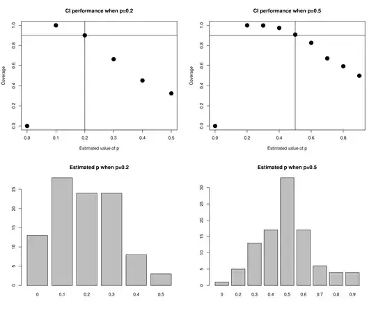
In the above examples, the mean coverage was pretty close to the desired coverage when true $p$=0.5 (87% compared with the desired 90%), but not so good when true $p$=0.2 (71% vs 90%).
# Compute mean coverage + other stats
summary(t2$coverage)
summary(t5$coverage)