5

I am performing survival analysis on credit data. I created a simple model with using interest rate:
cox <- coxph(Surv(periods,charged_off) ~ int_rate, data=notes) I assumed that int_rate was a time-independent variable, but the following test rejects HA:

> cox.zph(cox)
            rho chisq        p
int_rate 0.0446  14.2 0.000169

Same result for other variables such as loan amount:

> cox <- coxph(Surv(periods,charged_off) ~ int_rate + loan_amnt, data=notes)
> cox.zph(cox)
             rho chisq        p
int_rate  0.0364  9.31 2.28e-03
loan_amnt 0.0317  8.84 2.95e-03
GLOBAL        NA 26.28 1.97e-06

Plot for int_rate:

enter image description here

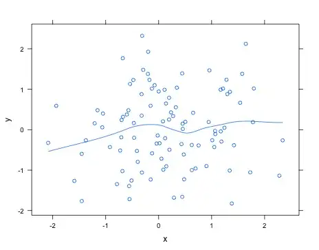
Why would these covariates be considered time dependent? Am I doing something wrong? Thanks.

Nick Stauner
  • 11,558
  • 5
  • 47
  • 105
John Richardson
  • 231
  • 4
  • 5
  • 2
    Although this question does not seem to call for a R solution, it remains good practice to flag that you are using R. – Nick Cox Jan 20 '14 at 15:46
  • Thanks for your attention, but I was suggesting flagging, not tagging. Look again at the R tag to see that the tag is needed only if the solution is to be R-based. Your question seems statistical. – Nick Cox Jan 20 '14 at 15:59
  • How large is your dataset? I notice the coefficient between transformed survival time and the scaled residuals, rho, is small. – Ellis Valentiner Jan 20 '14 at 16:14
  • 1
    I have over 240,000 observations. – John Richardson Jan 20 '14 at 16:26
  • Thinking about your data, why would you expect interest rate to be a time independent variable? The interest rate on a loan today is similar to what it was yesterday and will be tomorrow. In a month it may change slightly and in a year it will probably be noticeably different. Similarly the amount of my loan today is similar to that from last month, minus my monthly payment. – Ellis Valentiner Jan 20 '14 at 17:59
  • 1
    Graphically, you can see that there is a time-dependence (if there was none, your graph would be constant). That said, note that you should not overestimate the relevance of the $p$-value you get from `cox.zph`. This test is very sensitive, and will reject independence very quickly, even if that has little practical impact. Yes, your coefficients are significantly time-dependent, but *so what*? The $p$-value doesn't answer the real question, being how big a mistake you are making by treating the coefficient as time-independent (i.e., the effect size), or whether or not it matters at all. – Marc Claesen Oct 15 '15 at 14:05
  • I was once told that if you could fit a ruler between your error bands, that proportional hazards was a reasonable assumption. It may be a tight fit towards the right, but at least it isn't sinusoidal. – RayVelcoro Nov 04 '16 at 23:17

2 Answers2

1

The cox.zph function is measuring the overall effects of relaxing the assumption that the effect is constant in time. It telling you that the effect is probably not constant, but it's not telling you much more.

The plot is giving you further information about the time course and shows that the effect is maximal at intermediate values of time. I'm guessing that the outcome is loan default and that you are seeing a result that implies the probability of loan default is highest when the interest rate was high at loan origination and during intervals when the loan has been on the books for between 1 and 3 years. The impact of the interest rate then tapers off. This all seems perfectly sensible.

For further information on how the authors of the survival package use cox.zph, I recommend Chapter 6:"Testing Proportional Hazards" in their book, "Modeling Survival Data". Your result resembles their illustration of the time dependence of the Karnofsky performance measure. They consider various options for using a transformed time scale.

I wonder if you might have additional information such as the time-dependent covariate which would be the interest rates in periods after the loan origination?

DWin
  • 7,005
  • 17
  • 32
1

The distinction one has to make is between time-varying covariate and a covariate whose coefficient changes over time. Both violate the proportionality assumption, but do not have to be drawbacks. Rather, they can and are often theoretically meaningful (see Singer & Willett's book on Longitudinal Data Analysis and their 1991 paper in Psychological Bulletin). They just have to be included in the model.

In your plot, it looks like the coefficient for that time-invariant predictor changes over time (becomes less strong) and therefore violates the proportionality assumption. Including an interaction with that covariate and time would solve things and get around the proportionality assumption. Again, Singer and Willett's book is a classic--and highly accessible. The companion website also has code and examples for software implementation.

ATJ
  • 1,711
  • 1
  • 15
  • 20