11

Is there an easy way to apply the trend line formula from a chart to any given X value in Excel?

For example, I want to get the Y value for a given X = $2,006.00. I've already taken the formula and retyped it out be:

=-0.000000000008*X^3 - 0.00000001*X^2 + 0.0003*X - 0.0029

I am continually making adjustments to the trend line by adding more data, and don't want to retype out the formula every time.

enter image description here

Kirk Ouimet
  • 211
  • 1
  • 2
  • 7
  • Sounds like something a macro might accomplish, if you can find a person skilled enough in that. I know an inexpensive consultant that might be able to work that out for you. – rolando2 Mar 08 '11 at 23:11
  • @rolando You're right, but macros are unnecessary. Excel's LINEST will do it right in the sheet, which means it will dynamically update the results when the data change: that's even better than a macro :-). – whuber Mar 08 '11 at 23:46
  • Good to know. Thx. – rolando2 Mar 09 '11 at 23:22
  • 1
    Here is a link to a fuller list of Excel charting possibilites http://spreadsheetpage.com/index.php/tip/chart_trendline_formulas/ –  Mar 09 '11 at 18:34

2 Answers2

16

Use LINEST, as shown:

enter image description here

The method is to create new columns (C:E here) containing the variables in the fit. Perversely, LINEST returns the coefficients in the reverse order, as you can see from the calculation in the "Fit" column. An example prediction is shown outlined in blue: all the formulas are exactly the same as for the data.

Note that LINEST is an array formula: the answer will occupy p+1 cells in a row, where p is the number of variables (the last one is for the constant term). Such formulas are created by selecting all the output cells, pasting (or typing) the formula in the formula textbox, and pressing Ctrl-Shift-Enter (instead of the usual Enter).

whuber
  • 281,159
  • 54
  • 637
  • 1,101
  • Woah whuber, this is really, really helpful. Can you hook me up with a copy of that spreadsheet? – Kirk Ouimet Mar 09 '11 at 00:26
  • @Kirk You can create it yourself in no time. It's set up so by typing the formulas in C2:F2, you can drag them down as many rows as you like. Then type the LINEST formula in I2:L2. Just five simple formulas and you're done. – whuber Mar 09 '11 at 03:34
8

Try trend(known_y's, known_x's, new_x's, const).

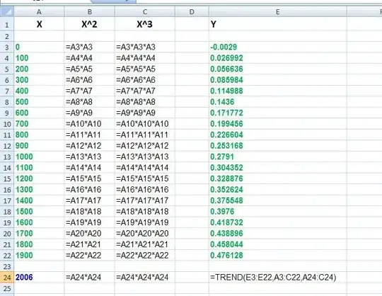
Column A below is X. Column B is X^2 (the cell to the left squared). Column C is X^3 (two cells to the left cubed). The trend() formula is in Cell E24 where the cell references are shown in red.

The "known_y's" are in E3:E22

The "known_x's" are in A3:C22

The "new_x's" are in A24:C24

The "const" is left blank.

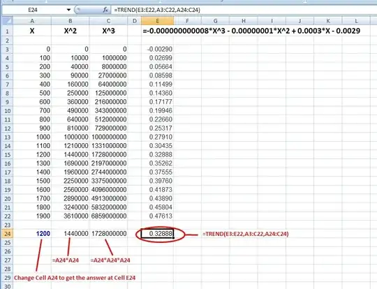
Cell A24 contains the new X, and is the cell to change to update the formula in E24

Cell B24 contains the X^2 formula (A24*A24) for the new X

Cell C24 contains the X^3 formula (A24*A24*A24) for the new X

If you change the values in E3:E22, the trend() function will update Cell E24 for your new input at Cell A24.

enter image description here

Edit ====================================

Kirk,

There's not much to the spreadsheet. I posted a "formula view" below.

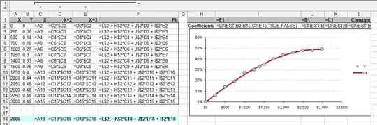
The "known_x" values are in green in A3:C22

The "known_y" values are in green in E3:E22

The "new_x" values are in cells A24:C24, where B24 and C24 are the formulas as shown. And, cell E24 has the trend() formula. You enter your new "X" in cell A24.

That's all there is to it.

enter image description here

bill_080
  • 3,458
  • 1
  • 20
  • 21