ARIMA estimation by hand

Question

I'm trying to understand how the parameters are estimated in ARIMA modeling/Box Jenkins (BJ). Unfortunately none of the books that I have encountered describes the estimation procedure such as Log-Likelihood estimation procedure in detail. Following is the Log-Likelihood for ARMA from any standard textbooks: $$ LL(\theta)=-\frac{n}{2}\log(2\pi) - \frac{n}{2}\log(\sigma^2) - \sum\limits_{t=1}^n\frac{e_t^2}{2\sigma^2} $$

I want to learn the ARIMA/BJ estimation by doing it myself. So I used $R$ to write a code for estimating ARMA by hand. Below is what I did in $R$,

• I simulated ARMA (1,1)
• Wrote the above equation as a function
• Used the simulated data and the optim function to estimate AR and MA parameters.
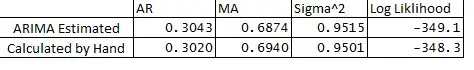
• I also ran the ARIMA in the stats package and compared the ARMA parameters from what I did by hand. Below is the comparison:

**Below are my questions:

• Why is there a slight difference between the estimated and calculated variables ?
• Does ARIMA function in R backcasts or does the estimation procedure differently than what is outlined below in my code?
• I have assigned e1 or error at observation 1 as 0, is this correct ?
• Also is there a way to estimate confidence bounds of forecasts using the hessian of the optimization ?

Thanks so much for your help as always.

Below is the code:

## Load Packages

library(stats)
library(forecast)

set.seed(456)


## Simulate Arima
y <- arima.sim(n = 250, list(ar = 0.3, ma = 0.7), mean = 5)
plot(y)

## Optimize Log-Likelihood for ARIMA

n = length(y) ## Count the number of observations
e = rep(1, n) ## Initialize e

logl <- function(mx){
  
  g <- numeric
  mx <- matrix(mx, ncol = 4)
  
  mu <- mx[,1] ## Constant Term
  sigma <- mx[,2] 
  rho <- mx[,3] ## AR coeff
  theta <- mx[,4] ## MA coeff
  
  e[1] = 0 ## Since e1 = 0
  
  for (t in (2 : n)){
    e[t] = y[t] - mu - rho*y[t-1] - theta*e[t-1]
  }
  
  ## Maximize Log-Likelihood Function 
  g1 <-  (-((n)/2)*log(2*pi) - ((n)/2)*log(sigma^2+0.000000001) - (1/2)*(1/(sigma^2+0.000000001))*e%*%e)
  
  ##note: multiplying Log-Likelihood by "-1" in order to maximize in the optimization
  ## This is done becuase Optim function in R can only minimize, "X"ing by -1 we can maximize
  ## also "+"ing by 0.000000001 sigma^2 to avoid divisible by 0
  g <- -1 * g1
  
  return(g)
  
}

## Optimize Log-Likelihood
arimopt <- optim(par=c(10,0.6,0.3,0.5), fn=logl, gr = NULL,
                 method = c("L-BFGS-B"),control = list(), hessian = T)
arimopt

############# Output Results###############
ar1_calculated = arimopt$par[3]
ma1_calculated = arimopt$par[4]
sigmasq_calculated = (arimopt$par[2])^2
logl_calculated = arimopt$val
ar1_calculated
ma1_calculated
sigmasq_calculated
logl_calculated

############# Estimate Using Arima###############
est <- arima(y,order=c(1,0,1))
est

Answer 1

There is the concept of exact likelihood. It requires the knowledge of initial parameters such as the fist value of the MA error (one of your questions). Implementations usually differ regarding how they treat the initial values. What I usually do is (which is not mentioned in many books) is to also maximize ML w.r.t. the initial values as well.

Please take a look at the following from Tsay, it is not covering all cases, but was quite helpful for me:

http://faculty.chicagobooth.edu/ruey.tsay/teaching/uts/lec8-08.pdf

Answer 2

Did you read the the help page of arima function? Here is the relevant excerpt:

The exact likelihood is computed via a state-space representation of the ARIMA process, and the innovations and their variance found by a Kalman filter. The initialization of the differenced ARMA process uses stationarity and is based on Gardner et al. (1980). For a differenced process the non-stationary components are given a diffuse prior (controlled by kappa). Observations which are still controlled by the diffuse prior (determined by having a Kalman gain of at least 1e4) are excluded from the likelihood calculations. (This gives comparable results to arima0 in the absence of missing values, when the observations excluded are precisely those dropped by the differencing.)

Also relevant is a parameter method=c("CSS-ML", "ML", "CSS"):

Fitting method: maximum likelihood or minimize conditional sum-of-squares. The default (unless there are missing values) is to use conditional-sum-of-squares to find starting values, then maximum likelihood.

Your results do not differ that much from the ones produced by arima function, so you definitely got everything right.

Remember that if you want to compare results of two optimisation procedures, you need to make sure, that the starting values are the same, and the same optimisation method is used, otherwise the results might differ.