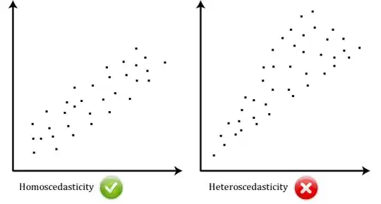
Homoskedasticity means that the variances of all the observations are identical to one another, heteroskedasticity means they're different. It's possible that the size of the variances displays some trend relative to x, but it's not strictly necessary; as shown in the accompanying diagram, variances that are differently sized in some random way from point to point will qualify just as well.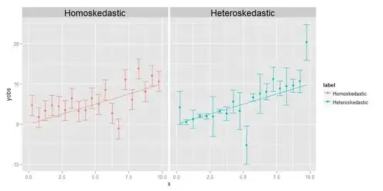
The job of the regression is to estimate an optimal curve which passes as close to as many of the data points as possible. In the case of heteroskedastic data, by definition some points will naturally be much more widely dispersed than others. If the regression simply treats all of the data points equivalently, the ones with the largest variance will tend to have undue influence in selecting the optimal regression curve, by "dragging" the regression curve toward themselves, in order to achieve the objective of minimizing the overall scatter of the data points about the final regression curve.
This issue can easily be overcome by simply weighting each data point in inverse proportion to its variance. This assumes, however, that one knows the variance associated with each individual point. Often, one doesn't. Thus, the reason that homoskedastic data are preferred is because they are simpler and easier to deal with--you can get the "correct" answer for the regression curve without necessarily knowing the underlying variances of the individual points, because the relative weights between the points in some sense will "cancel out" if they are all the same anyway.
EDIT:
A commenter asks me to explain the idea that individual points may have their own, unique, different variances. I do so with a thought experiment. Suppose I ask you to measure the weight vs. length of a bunch of different animals, from the size of a gnat all the way up to the size of an elephant. You do so, plotting length on the x-axis, and weight on the y-axis. But let's pause for a moment to consider things in a little more detail. Let's look at the weight values specifically--how did you actually obtain them? You can't possibly use the same physical measuring device to weigh a gnat as you would to weigh a house pet, nor can you use the same device to weigh a house pet as you would to weigh an elephant. For the gnat, you are probably going to have to use something like an analytical chemistry balance, accurate down to 0.0001 g, while for the house pet, you'd use a bathroom scale, which might be accurate to about a half of a pound or so (roughly around 200 g), while for the elephant, you might use a something like a truck scale, which might only be accurate to within +/- 10 kg. The point is, all of these devices have different inherent accuracies--they only tell you the weight up to a certain number of significant digits, and after that you can't really know for sure. The different sizes of the error bars in the heteroskedastic plot above, which we associate with the different variances of the individual points, reflect differing degrees of certainty about the underlying measurements. In short, different points can have different variances because sometimes we can't measure all of the points equally well--you're never going to know the weight of an elephant down to +/- 0.0001 g, because you can't get that kind of accuracy out of a truck scale. But you can know the weight of a gnat to +/- 0.0001 g, because you can get that kind of an accuracy on an analytical chemistry balance. (Technically, in this particular thought experiment, the same type of issue actually arises for the length measurement as well, but all that really means is that if we decided to plot horizontal error bars representing uncertainties in the x-axis values also, those would have different sizes for different points too.)