7

In To P or not to P: on the evidential nature of P-values and their place in scientic inference, Michael Lew has shown that, at least for the t-test, the one-sided p-value and sample size can be interpreted as an "address" (my term) for a given likelihood function. I have repeated some of his figures below with slight modification. The left column shows the distribution of p-values expected due to theory for different effect sizes (difference between means/pooled sd) and sample sizes. The horizontal lines mark the "slices" from which we get the likelihood functions shown by the right panels for p=0.50 and p=0.025.

enter image description here

These results are consistent with monte carlo simulations. For this figure I compared two groups with n=10 via t-test at a number of different effect sizes and binned 10,000 p-values into .01 intervals for each effect size. Specifically there was one group with mean=0, sd=1 and a second with a mean that I varied from -4 to 4, also with sd=1. enter image description here

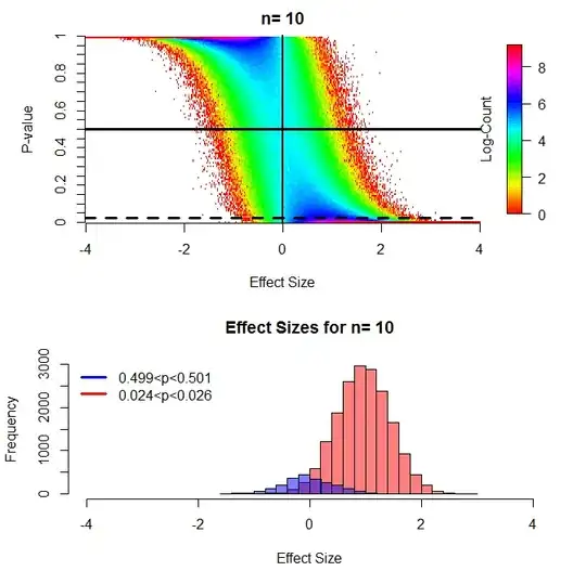
(The above figures can be directly compared to figures 7/8 from the paper linked above and are very similar, I found the heatmaps more informative than the "clouds" used in that paper and also wished to independently replicate his result.)

If we examine the likelihood functions "indexed" by the p-values, the behaviour of rejecting/accepting hypotheses or ignoring results giving p-values greater than 0.05 based on a cut-off value (either the arbitrary 0.05 used everywhere or determined by cost-benefit) appears to be absurd. Why should I not conclude from the n=100, p=0.5 case that "the current evidence shows that any effect, if present, is small"? Current practice would be to either "accept" there is no effect (hypothesis testing) or say "more data needed" (significance testing). I fail to see why I should do either of those things.

Perhaps when a theory predicted a precise point value, then rejecting a hypothesis could make sense. But when the hypotheses are of the form either "mean1=mean2 or mean1!=mean2" I see no value. Under the conditions these tests are often being used randomization does not guarantee all confounds are balanced across groups and there should always be the worry of lurking variables, so rejecting the hypothesis that mean1 exactly equals mean2 has no scientific value as far as I can tell.

Are there cases beyond the t-test where this argument would not apply? Am I missing something of value that rejecting a hypothesis with low a priori probability provides to researchers? Ignoring results above an arbitrary cutoff seems to have lead to widespread publication bias. What useful role does ignoring results play for scientists?

Michael Lew's R code to calculate the p-value distributions

LikeFromStudentsTP<-function(n,x,Pobs,test.type, alt='one.sided'){
# test.type can be 'one.sample', 'two.sample' or 'paired'
# n is the sample size (per group for test.type = 'two.sample')
# Pobs is the observed P-value
# h is a small number used in the trivial differentiation
h<-10^-7
PowerDn<-power.t.test('n'=n, 'delta'=x, 'sd'=1,
'sig.level' = Pobs-h, 'type'= test.type, 'alternative'=alt)
PowerUp<-power.t.test('n'=n, 'delta'=deltaOnSigma, 'sd'=1,
'sig.level' = Pobs+h, 'type'= test.type, 'alternative'=alt)
PowerSlope<-(PowerUp$power-PowerDn$power)/(h*2)
L<-PowerSlope
}

R code for figure 1

deltaOnSigma <- 0.01*c(-400:400)
type<-'two.sample'
alt='one.sided'
p.vals<-seq(0.001,.999,by=.001)


#dev.new()
par(mfrow=c(4,2))
for(n in c(3,5,10,100)){

  m<-matrix(nrow=length(deltaOnSigma), ncol=length(p.vals))
  cnt<-1
  for(P in p.vals){
    m[,cnt]<-LikeFromStudentsTP(n,deltaOnSigma,P,type, alt)
    cnt<-cnt+1
  }

  #remove very small values
  m[which(m/max(m,na.rm=T)<10^-5)]<-NA


  m2<-log(m)

  par(mar=c(4.1,5.1,2.1,2.1))
  image.plot(m2, axes=F,
             breaks=seq(min(m2, na.rm=T),max(m2, na.rm=T),length=1000), col=rainbow(999),
             xlab="Effect Size", ylab="P-value"
  )
  title(main=paste("n=",n))
  axis(side=1, at=seq(0,1,by=.25), labels=seq(-4,4,by=2))
  axis(side=2, at=seq(0,1,by=.05), labels=seq(0,1,by=.05))
  axis(side=4, at =.5, labels="Log-Likelihood", pos=.95, tick=F)
  abline(v=0.5, lwd=1)
  abline(h=.5, lwd=3, lty=1)
  abline(h=.025, lwd=3, lty=2)
  par(mar=c(5.1,4.1,4.1,2.1))


  plot(deltaOnSigma,m[,which(p.vals==.025)], type="l", lwd=3, lty=2,
       xlab="Effect Size", ylab="Likelihood", xlim=c(-4,4),
       main=paste("Likelihood functions for","n=",n)
  )
  lines(deltaOnSigma,m[,which(p.vals==.5)], lwd=3, lty=1)
  legend("topleft", legend=c("p=.5","p=.025"), lty=c(1,2),lwd=1, bty="n")
}

R code for figure 2

p.vals<-seq(0,1,by=.01)
deltaOnSigma <- 0.01*c(-400:400)
n<-10
n2<-10
sd2<-1
num.sims<-10000
sp<-sqrt((9*1^2 +(n2-1)*sd2^2)/(n+n2-2))

p.out=matrix(nrow=num.sims*length(deltaOnSigma) ,ncol=2)
m<-matrix(0,nrow=length(deltaOnSigma),ncol=length(p.vals))
pb<-txtProgressBar(min = 0, max = length(deltaOnSigma) ,style = 3)
cnt<-1
cnt2<-1
for(i in deltaOnSigma ){

  for(j in 1:num.sims){

    m2<-i
    a<-rnorm(n,0,1)
    b<-rnorm(n,m2,sd2)
    p<-t.test(a,b, alternative="less")$p.value

    r<-end(which(deltaOnSigma<=m2/sp))[1]

    m[r,end(which(p.vals<p))[1]]<-m[r,end(which(p.vals<p))[1]]+1
    p.out[cnt,]<-cbind(m2/sp,p)
    cnt<-cnt+1

  }
  cnt2<-cnt2+1
  setTxtProgressBar(pb, cnt2)
}
close(pb)


m[which(m==0)]<-NA

m2<-log(m)


dev.new()
par(mfrow=c(2,1))
par(mar=c(4.1,5.1,2.1,2.1))
image.plot(m2, axes=F,
           breaks=seq(min(m2, na.rm=T),max(m2, na.rm=T),length=1000), col=rainbow(999),
           xlab="Effect Size", ylab="P-value"
)
title(main=paste("n=",n))
axis(side=1, at=seq(0,1,by=.25), labels=seq(-4,4,by=2))
axis(side=2, at=seq(0,1,by=.05), labels=seq(0,1,by=.05))
axis(side=4, at =.5, labels="Log-Count", pos=.95, tick=F)
abline(h=.5, lwd=3, lty=1)
abline(h=.025, lwd=3, lty=2)
abline(v=.5, lwd=2, lty=1)
par(mar=c(5.1,4.1,4.1,2.1))


hist(p.out[which(p.out[,2]>.024 & p.out[,2]<.026),1],
     xlim=c(-4,4), xlab="Effect Size", col=rgb(1,0,0,.5), 
     main=paste("Effect Sizes for","n=",n)
)
hist(p.out[which(p.out[,2]>(.499) & p.out[,2]<.501),1], add=T,
     xlim=c(-4,4),col=rgb(0,0,1,.5)
)

legend("topleft", legend=c("0.499<p<0.501","0.024<p<0.026"), 
       col=c("Blue","Red"), lwd=3, bty="n")
Flask
  • 1,711
  • 1
  • 14
  • 24
  • As much as I like the discussion topic, this question is very broad and seems to be requesting opinions. As such, it's off topic for Cross Validated. Is your question the title or all of the many questions within? – John Nov 06 '13 at 11:51
  • @John In my experiance when it it comes to statistics I am bad at asking exactly the question that I want an answer to. So I place a general question as the the title and a number of "sub-questions" that have lead me to ask the general question within the body of the text. I do not mean to request opinions, however, if there is no non-opinionated answer to this basic question that underlies all of current applied statistics I think that itself would make for an appropriate answer. – Flask Nov 06 '13 at 12:04
  • The answer to your title question is a book in and of itself and the rest of the question mostly invites opinion. Hopefully informed opinion but it seems to be testing the paper cited. I'm all for this discussion, it's just that this isn't the place for it. I'm voting to close but could be persuaded otherwise. (my 2¢ on the paper is that I appreciate much of the argument but section 4.1 makes a grave error because p-values generated from data peeking with low N are no longer random variables but cherry picked p-values.) – John Nov 06 '13 at 12:54
  • I had not looked at the rules before but would argue that this question does ['inspire answers that explain “why” and “how”'](http://stats.stackexchange.com/help/dont-ask) – Flask Nov 06 '13 at 13:00
  • (ammendment to prior 2¢ *reported* p-values would not be unbiased random variables...you've gone through the garden and picked the best cherries.) – John Nov 06 '13 at 13:15
  • @John I agree that the wider framework in which these results are presented is not really established. However, I found the definition of p-value presented in this paper to be quite enlightening and it is this aspect that so clearly let me understand the evidence I would be ignoring by following significance testing protocol. – Flask Nov 06 '13 at 20:30
  • @John, also I disagree with your claim that the answer must be a book in and of itself. I provided an answer due to my understanding within the question. It is appropriate to reject an hypothesis when it has been predicted by theory or "common sense". Most early uses of p-values were of this type. Coming up with a statistical hypothesis just to be able to reject something is what does not seem reasonable. If I know so little that my theory cannot predict anything the best thing seems to be to simply describe the data/methods and share it with others until someone does come up with a theory. – Flask Nov 06 '13 at 21:07
  • An opinion answer would be short. An informed contrary opinion that dealt with the extensive arguments here and in the referred paper would be very long and broad. Neither answer is appropriate for the site. – John Nov 07 '13 at 00:15
  • @John I still believe this question meets the criteria put forward in the help page. It also says good questions "tend to have long, not short, answers". It should not take a book to explain when it makes sense to perform acceptance/rejection procedures. For example, I found the current answer helpful and it is not book-length. – Flask Nov 07 '13 at 01:31

1 Answers1

1

I really like your rainbow versions of my clouds, and may 'borrow' them for a future version of my paper. Thank you!

Your questions are not entirely clear to me, so I will paraphrase them. If they are not what you had in mind them my answers will be misdirected!

  • Are there situations where rejection of the hypothesis like "mean1 equals mean2" is scientifically valuable?

Frequentists would contend that the advantage of having well-defined error rates outweighs the loss of assessment of evidence that comes with their methods, but I don't think that that is very often the case. (And I would suspect that few proponents of the methods really understand the complete loss of evidential consideration of the data that they entail.) Fisher was adamant that the Neyman-Pearson approach to testing had no place in a scientific program, but he did allow that they were appropriate in the situation of 'industrial acceptance testing'. Presumably such a setting is a situation where rejection of a point hypothesis can be useful.

Most of science is more accurately modelled as estimation than as an acceptance procedure. P-values and the likelihood functions that they index (or, to use your term, address) provide very useful information for estimation, and for inferences based on that estimation.

(A couple of old StackExchange questions and answerd are relevant: What is the difference between "testing of hypothesis" and "test of significance"? and Interpretation of p-value in hypothesis testing)

  • Are you missing the point of rejection of a hypothesis (of low a priori probability)?

I don't know if you are missing much, but it is probably not a good idea to add prior probabilities into this mixture! Much of the argumentation around the ideas relating to hypothesis testing, significance testing and evidential evaluation come from entrenched positions. Such arguments are not very helpful. (You might have noticed how carefully I avoided bringing Bayesianism into my discussion in the paper, even though I wholeheartedly embrace it when there are reasonable prior probabilities to use. First we need to fix the P-value provide evidence, error rates do not issue.)

  • Should scientists ignore results that fail to reach 'significance'?

No, of course not. Using an arbitrary cutoff to claim significance, or to assume significance, publishability, repeatability or reality of a result is a bad idea in most situations. The results of scientific experiments should be interpreted in light of prior understanding, prior probabilities where available, theory, the weight of contrary and complementary evidence, replications, loss functions where appropriate and a myriad of other intangibles. Scientists should not hand over to insentient algorithms the responsibility for inference. However, to make full use of the evidence within their experimental results scientists will need to much better understand what the statistical analyses can and do provide. That is the purpose of the paper that you have explored. It will also be necessary that scientists make a more complete account of their acquisition of evidence and the evolution of their understanding than what is usually presented in papers, and they should provide what Abelson called a principled argument to support their inferences. Relying on P<0.05 is the opposite of a principled argument.

Michael Lew
  • 10,995
  • 2
  • 29
  • 47
  • As far as I can tell the frequentist approach is simply not compatible with the realities of performing science. It results in various absurdities/misunderstandings such as "don't check your results until the study is over" (yes, this is what I believed). But you seem to already agree with this so I would like someone else's opinion. Second, it is difficult for me to imagine someone defending a high prior probability that two group averages are exactly equal if they are asked explicitly. I do not think this is necessarily a "Bayesian" point of view. – Flask Nov 06 '13 at 05:34
  • Flask, perhaps you mean NHST rather than the "frequentist approach"? There are several frequentist approaches. – John Nov 06 '13 at 13:00
  • @John I cannot say I am aware of the hierarchy of approaches towards statistics (this would be a useful paper/site...). When I think frequentist, I think of it in direct contrast from what I have read by Fisher, things like "accept an hypothesis" and "long run". My background is disgruntled NHST hybrid victim, so I am sure this has influenced what I have been exposed to. – Flask Nov 06 '13 at 13:17
  • Fisher is in the frequentist family. So, you really mean NHST since (and a mishmash of Fisher and Neyman-Pearson). – John Nov 06 '13 at 13:27
  • @John I don't think so, but I will perhaps ask a question on this later. – Flask Nov 06 '13 at 13:46
  • 1
    @John Fisher is often assumed to be a Frequentist, but his allegiances are much more complicated than that. He derided the Neyman-Pearson approach at every opportunity, after a short initial period of acceptance, and his later writings made it quite clear that he was interested in the evidential nature of the data, something that is excluded from Frequentism. He is probably better characterised as a likelihoodist and, depending on how one takes his fiducial argument, a closet Bayesian in denial. If you are interested in Fisher then you need to be quite careful with secondary sources. – Michael Lew Nov 06 '13 at 19:35
  • I'd be happy to justify a different category for later career Fisher (but the Bayesians can't just adopt him post hoc :)). Nevertheless, N-P, confidence intervals, and other frequentist statistics have quite well contained and reasonable arguments. It's NHST that is foundationless. I also agree there are large areas of science for which N-P really is the wrong approach. But it is quite helpful in others and just shouldn't be equated with NHST. As an aside Michael, I'd be more than happy to provide some helpful comments on the article if you're open to revision...not sure how to go to chat. – John Nov 07 '13 at 00:25
  • @John If you want to chat, just email me, I'd be pleased. My address is in the paper that is cited in the original post. – Michael Lew Nov 07 '13 at 00:37