The connection between Bayesian statistics and generative modeling

Question

Can someone refer me to a good reference that explains the connection between Bayesian statistics and generative modeling techniques? Why do we usually use generative models with Bayesian techniques?

Why it is especially appealing to use Bayesian statistics in the absence of complete data, if at all?

Note that I come from a more machine learning oriented view, and I am interested in reading more about it from the statistics community.

Any good reference that discusses these points would be greatly appreciated. Thanks.

Answer 1

In machine learning a full probability model p(x,y) is called generative because it can be used to generate the data whereas a conditional model p(y|x) is called discriminative because it does not specify a probability model for p(x) and can only generate y given x. Both can be estimated in Bayesian fashion.

Bayesian estimation is inherently about specifying a full probability model and performing inference conditional on the model and data. That makes many Bayesian models have a generative feel. However to a Bayesian the important distinction is not so much about how to generate the data, but more about what is needed to obtain the posterior distribution of the unknown parameters of interest.

The discriminative model p(y|x) is part of bigger model where p(y, x) = p(y|x)p(x). In many instances, p(x) is irrelevant to the posterior distribution of the parameters in the model p(y|x). Specifically, if the parameters of p(x) are distinct from p(y|x) and the priors are independent, then the model p(x) contains no information about the unknown parameters of the conditional model p(y|x), so a Bayesian does not need to model it.

---

At a more intuitive level, there is a clear link between "generating data" and "computing the posterior distribution." Rubin (1984) gives the following excellent description of this link:

---

Bayesian statistics is useful given missing data primarily because it provides a unified way to eliminate nuisance parameters -- integration. Missing data can be thought of as (many) nuisance parameters. Alternative proposals such as plugging in the expected value typically will perform poorly because we can rarely estimate missing data cells with high levels of accuracy. Here, integration is better than maximization.

Discriminative models like p(y|x) also become problematic if x includes missing data because we only have data to estimate p(y|x_obs) but most sensible models are written with respect to the complete data p(y|x). If you have a fully probability model p(y,x) and are Bayesian, then you're fine because you can just integrate over the missing data like you would any other unknown quantity.

Answer 2

@Tristan: Hope you don't mind my reworking of you answer as I am working on how to make the general point as transparent as possible.

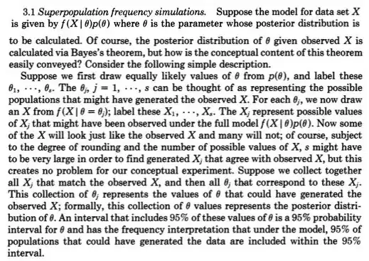
To me, the primary insight in statistics is to conceptualize repeated observations that vary - as being generated by a probability generating model, such as Normal(mu,sigma). Early in the 1800,s the probability generating models entertained were usually just for errors of measurement with the role of parameters, such as mu and sigma and priors for them muddled. Frequentist approaches took the parameters as fixed and unknown and so the probability generating models then only involved possible observations. Bayesian approaches (with proper priors) have probability generating models for both possible unknown parameters and possible observations. These joint probability generating models comprehensively account for all of the - to put it more generally - possible unknowns (such as parameters) and knowns (such as observations). As in the link from Rubin you gave, conceptually Bayes theorem states only keep the possible unknowns that (in the simulation) actually generated possible knowns that were equal (very close) to the actual knowns (in your study).

This actually was very clearly depicted by Galton in a two stage quincunx in the late 1800,s. See figure 5 > Stigler, Stephen M. 2010. Darwin, Galton and the statistical

enlightenment. Journal of the Royal Statistical Society: Series A 173(3):469-482. .

It is equivalent but perhaps more transparent that

posterior = prior(possible unknowns| possible knowns=knowns)

than posterior ~ prior(possible unknowns)*p(possible knowns=knowns|possible unknowns)

Nothing much new for missing values in the former as one just adds possible unknowns for a probability model generating missing values and treats missing as just one of the possible knowns (i.e. the 3rd observation was missing).

Recently, approximate Bayesian computation (ABC) has taken this constructive two-stage simulation approach seriously when p(possible knowns=knowns|possible unknowns) cannot be worked out. But even when this can be worked out and the posterior easily obtainable from MCMC sampling (or even when the posterior is directly available due to the prior being conjugate) Rubin’s point about this two-stage sampling construction enabling easier understanding, should not be overlooked.

For instance, I am sure it would have caught what @Zen did here Bayesians: slaves of the likelihood function? because one would needed to draw a possible unknown c from a prior (stage one) and then draw a possible known (data) given that c (stage 2) which would not have been a random generation as p(possible knowns|c) would not have been be a probability except for one and only one c.

From @Zen “Unfortunatelly, in general, this is not a valid description of a statistical model. The problem is that, by definition, $f_{X_i\mid C}(\,\cdot\mid c)$ must be a probability density for almost every possible value of $c$, which is, in general, clearly false.”