The tail dependence coefficients $\lambda_U$ and $\lambda_L$ are measures of extremal dependence that quantify the dependence in the upper and lower tails of a bivariate distribution with continuous margins $F$ and $G$.
The coefficients $\lambda_U$ and $\lambda_L$ are defined in terms of quantile exceedences.
For the upper tail dependence coefficient $\lambda_U$ one looks at the probability that $Y$ exceeds the $u$-quantile $G^{-1}(u)$, given that $X$ exceeds the $u$-quantile $F^{-1}(u)$, and then consider the limit as $u$ goes to $1$, provided it exists.
Large values of $\lambda_U$ imply that joint extremes are more likely than for low values of $\lambda_U$. Interpretation for the lower tail dependence coefficient $\lambda_L$ is analogous.
If $\lambda_U = 0$, then $X$ and $Y$ are said to be asymptotically independent; if $\lambda_U \in (0, 1]$ they are asymptotically dependent.
For independent variables $\lambda_U = 0$; for perfectly dependent variables $\lambda_U = 0$. Note that $\lambda_U = 0$ does NOT imply independence; the comment/statement in the question's reference is wrong. Indeed, consider a bivariate normal distribution with correlation $\rho \notin \{0, 1\}$. Then, one can show that $\lambda_U = 0$ but the variables are dependent.
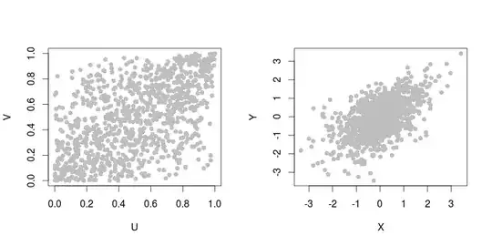
A distribution with, say, $\lambda_U = 0.5$ does not mean that there is a linear dependence between $X$ and $Y$; it means that $X$ and $Y$ are asymptotically dependent in the upper tail, and the strength of the dependence is 0.5. For example, the Gumbel copula with parameter $\theta = \log(2)/\log(1.5)$ has
a coefficient of upper tail dependence equal to $0.5$.
The following figure shows a sample of 1000 points of the Gumbel copula with parameter $\theta = \log(2)/\log(1.5)$ with uniform margins (left) and standard normal margins (right). The data were generated with the copula package in R (code is provided below).
## Parameters
theta <- log(2)/log(1.5)
n     <- 1000

## Generate a sample
library(copula)
set.seed(234)
gumbel.cop <- archmCopula("gumbel", theta)
x <- rCopula(n, gumbel.cop)

## Visualization
par(mfrow = c(1, 2))
plot(x, pch = 16, col = "gray", xlab = "U", ylab = "V")
plot(qnorm(x), pch = 16, col = "gray", xlab = "X", ylab = "Y")
par(mfrow = c(1, 1))