How to include a linear and quadratic term when also including interaction with those variables?

Question

When adding a numeric predictor with categorical predictors and their interactions, it is usually considered necessary to center the variables at 0 beforehand. The reasoning is that the main effects are otherwise hard to interpret as they are evaluated with the numeric predictor at 0.

My question now is how to center if one not only includes the original numeric variable (as a linear term) but also the quadratic term of this variable? Here, two different approaches are necessary:

1. Centering both variables at their individual mean. This has the unfortunate downside that the 0 now is at a different position for both variables considering the original variable.
2. Centering both variables at the mean of the original variable (i.e., subtracting the mean from the original variable for the linear term and subtracting the square of the mean of the original variable from the quadratic term). With this approach the 0 would represent the same value of the original variable, but the quadratic variable would not be centered at 0 (i.e., the mean of the variable wouldn't be 0).

I think that approach 2 seems reasonable given the reason for centering after all. However, I cannot find anything about it (also not in the related questions: a and b).

Or is it generally a bad idea to include linear and quadratic terms and their interactions with other variables in a model?

Answer 1

When including polynomials and interactions between them, multicollinearity can be a big problem; one approach is to look at orthogonal polynomials.

Generally, orthogonal polynomials are a family of polynomials which are orthogonal with respect to some inner product.

So for example in the case of polynomials over some region with weight function $w$, the inner product is $\int_a^bw(x)p_m(x)p_n(x)dx$ - orthogonality makes that inner product $0$ unless $m=n$.

The simplest example for continuous polynomials is the Legendre polynomials, which have constant weight function over a finite real interval (commonly over $[-1,1]$).

In our case, the space (the observations themselves) is discrete, and our weight function is also constant (usually), so the orthogonal polynomials are a kind of discrete equivalent of Legendre polynomials. With the constant included in our predictors, the inner product is simply $p_m(x)^Tp_n(x) = \sum_i p_m(x_i)p_n(x_i)$.

For example, consider $x = 1,2,3,4,5$

Start with the constant column, $p_0(x) = x^0 = 1$. The next polynomial is of the form $ax-b$, but we're not worrying about scale at the moment, so $p_1(x) = x-\bar x = x-3$. The next polynomial would be of the form $ax^2+bx+c$; it turns out that $p_2(x)=(x-3)^2-2 = x^2-6x+7$ is orthogonal to the previous two:

x         p0  p1  p2   
1          1  -2   2   
2          1  -1  -1
3          1   0  -2
4          1   1  -1
5          1   2   2

Frequently the basis is also normalized (producing an orthonormal family) - that is, the sums of squares of each term is set to be some constant (say, to $n$, or to $n-1$, so that the standard deviation is 1, or perhaps most frequently, to $1$).

Ways to orthogonalize a set of polynomial predictors include Gram-Schmidt orthogonalization, and Cholesky decomposition, though there are numerous other approaches.

---

Some of the advantages of orthogonal polynomials:

1) multicollinearity is a nonissue - these predictors are all orthogonal.

2) The low-order coefficients don't change as you add terms. If you fit a degree $k$ polynomial via orthogonal polynomials, you know the coefficients of a fit of all the lower order polynomials without re-fitting.

---

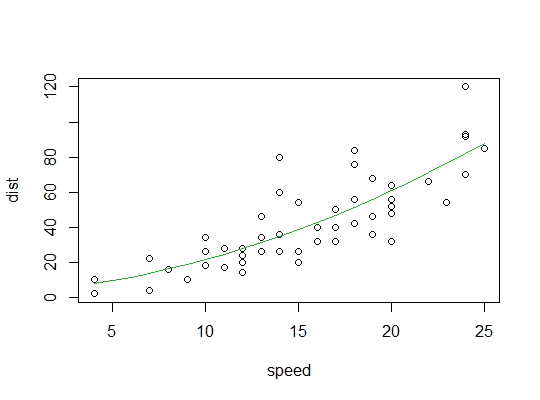
Example in R (cars data, stopping distances against speed):

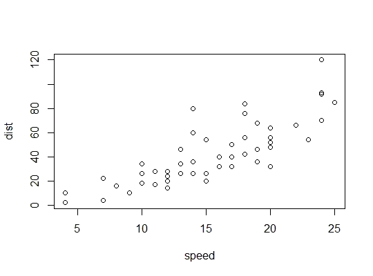
Here we consider the possibility that a quadratic model might be suitable:

R uses the poly function to set up orthogonal polynomial predictors:

> p <- model.matrix(dist~poly(speed,2),cars)
> cbind(head(cars),head(p))
  speed dist (Intercept) poly(speed, 2)1 poly(speed, 2)2
1     4    2           1      -0.3079956      0.41625480
2     4   10           1      -0.3079956      0.41625480
3     7    4           1      -0.2269442      0.16583013
4     7   22           1      -0.2269442      0.16583013
5     8   16           1      -0.1999270      0.09974267
6     9   10           1      -0.1729098      0.04234892

They're orthogonal:

> round(crossprod(p),9)
                (Intercept) poly(speed, 2)1 poly(speed, 2)2
(Intercept)              50               0               0
poly(speed, 2)1           0               1               0
poly(speed, 2)2           0               0               1

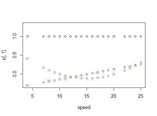
Here's a plot of the polynomials:

Here's the linear model output:

> summary(carsp)

Call:
lm(formula = dist ~ poly(speed, 2), data = cars)

Residuals:
    Min      1Q  Median      3Q     Max 
-28.720  -9.184  -3.188   4.628  45.152 

Coefficients:
                Estimate Std. Error t value Pr(>|t|)    
(Intercept)       42.980      2.146  20.026  < 2e-16 ***
poly(speed, 2)1  145.552     15.176   9.591 1.21e-12 ***
poly(speed, 2)2   22.996     15.176   1.515    0.136    
---
Signif. codes:  0 ‘***’ 0.001 ‘**’ 0.01 ‘*’ 0.05 ‘.’ 0.1 ‘ ’ 1

Residual standard error: 15.18 on 47 degrees of freedom
Multiple R-squared:  0.6673,    Adjusted R-squared:  0.6532 
F-statistic: 47.14 on 2 and 47 DF,  p-value: 5.852e-12

Here's a plot of the quadratic fit:

Answer 2

I don't feel that centering is worth the trouble, and centering makes the interpretation of parameter estimates more complex. If you use modern matrix algebra software, algebraic collinearity is not a problem. Your original motivation of centering to be able to interpret main effects in the presence of interaction is not a strong one. Main effects when estimated at any automatically chosen value of a continuous interacting factor are somewhat arbitrary, and it's best to think of this as a simple estimation problem by comparing predicted values. In the R rms package contrast.rms function, for example, you can obtain any contrast of interest independent of variable codings. Here is an example of a categorical variable x1 with levels "a" "b" "c" and a continuous variable x2, fitted using a restricted cubic spline with 4 default knots. Different relationships between x2 and y are allowed for different x1. Two of the levels of x1 are compared at x2=10.

require(rms)
dd <- datadist(x1, x2); options(datadist='dd')
f <- ols(y ~ x1 * rcs(x2,4))
contrast(f, list(x1='b', x2=10), list(x1='c', x2=10))
# Now get all comparisons with c:
contrast(f, list(x1=c('a','b'), x2=10), list(x1='c', x2=10))
# add type ='joint' to get a 2 d.f. test, or conf.type='simultaneous'
# to get simultaneous individual confidence intervals

With this approach you can also easily estimate contrasts at several values of the interacting factor(s), e.g.

contrast(f, list(x1='b', x2=10:20), list(x1='c', x2=10:20))