11

I have been given this task and was stumped. A colleague asked me to estimate the $x_{upper}$ and $x_{lower}$ of the following chart:

enter image description here

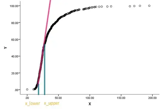
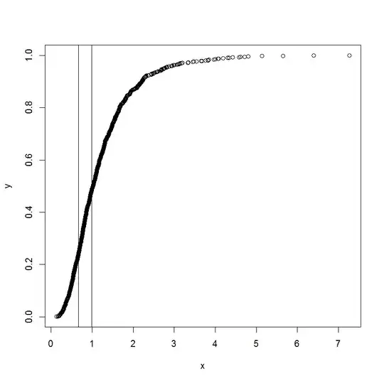
The curve is actually a cumulative distribution, and x is some kind of measurements. He is interested to know what are the corresponding values on x when the cumulative function started to become straight and deviate from being straight.

I understand that we can use differentiation to find the slope at a point, but I am not too sure how to determine when can we call the line straight. Any nudge towards some already existing approach/literature will be greatly appreciated.

I know R as well if you happen to know any relevant packages or examples on this kind of investigations.

Thanks a lot.


UPDATE

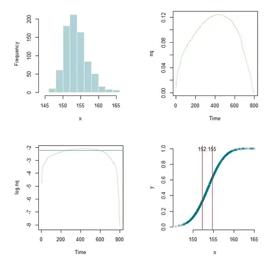
Thanks to Flounderer I was able to expand the work further, set up a framework, and tinker the parameters here and there. For learning purpose here are my current code and a graphic output.

library(ESPRESSO)

x <- skew.rnorm(800, 150, 5, 3)
x <- sort(x)
meanX <- mean(x)
sdX <- sd(x)
stdX <- (x-meanX)/sdX
y <- pnorm(stdX)

par(mfrow=c(2,2), mai=c(1,1,0.3,0.3))
hist(x, col="#03718750", border="white", main="")

nq <- diff(y)/diff(x)
plot.ts(nq, col="#6dc03480")

log.nq <- log(nq)
low <- lowess(log.nq)
cutoff <- .7
q <- quantile(low$y, cutoff)
plot.ts(log.nq, col="#6dc03480")
abline(h=q, col="#348d9e")

x.lower <- x[min(which(low$y > q))]
x.upper <- x[max(which(low$y > q))]
plot(x,y,pch=16,col="#03718750", axes=F)
axis(side=1)
axis(side=2)
abline(v=c(x.lower, x.upper),col="red")
text(x.lower, 1.0, round(x.lower,0))
text(x.upper, 1.0, round(x.upper,0))

enter image description here

amoeba
  • 93,463
  • 28
  • 275
  • 317
Penguin_Knight
  • 11,078
  • 29
  • 48
  • 2
    Can you try to determine when the second derivative is 0 or close to 0? – alex Oct 09 '13 at 21:05
  • 3
    The problem of formulation can be that - quite likely - the "straight" cut does not exist. If you take a strong lens and inspect that region you might notice that it is still smoothly S-shaped. – ttnphns Oct 09 '13 at 21:09
  • @alex Thanks for this tip, I'll roll up my sleeves and give it some thoughts and a try. – Penguin_Knight Oct 09 '13 at 21:13
  • @ttnphns Do understand. I'm also aware that just by stretching the axes the perception can change as well... that's why I suggested consulting crowd for a quantitative alternative rather than visually defining the values. – Penguin_Knight Oct 09 '13 at 21:16
  • 2
    If one were to fit some density (say by kernel density estimation, log-spline density estimation, or even some parametric model), the height of the density at its peak is an estimate of the maximum slope of the CDF. The 'breadth' of the peak tells you something about how wide the range of the x-values is where it makes some kind of sense to talk about that slope as if it were constant. – Glen_b Oct 10 '13 at 00:44
  • Than you @Glen_b. Yes, I do believe he realizes that. The researcher is curious to compare this range obtained from a subpopulation with the population range. The general premise is to find out if we can learn anything about population's reference values just by looking at special subgroups, such as the sick or institutionalized. – Penguin_Knight Oct 10 '13 at 01:29
  • 2
    To follow up on @Glen_b's comment, the main point is that what you are asking for has not been defined with sufficient rigor. Just how far below the maximum of the PDF should the "shoulders" x_lower and x_upper be located? Some quantitative criterion is needed. – whuber Oct 10 '13 at 16:47
  • @whuber, thanks of the comment. I understand that the challenge is to define how different is different. I will propose this method to them with some warning, and may also tag along a couple other suggestions such as SD or a trimmed distribution, etc. – Penguin_Knight Oct 10 '13 at 20:51
  • Why does your colleague want to know? Is it just to be able to use a good-enough linear approximation for part of the curve, or are $x_low$ & $x_high$ going to be used for any special purposes? – Scortchi - Reinstate Monica Oct 11 '13 at 08:54
  • @Scortchi, the latter one. They were checking the data and accidentally plotted the accumulative frequency of a biomedical outcome of an institutionalized group (probably nursing home/hospital). Visually, they found that the beginning and the end of the straight portion seemed to align with the population-based normal range. This sparked their interest to learn more about this phenomenon. I'm skeptical, but also think that it'd be a good exercise to actually apply this technique to other variables and see what comes out of it. – Penguin_Knight Oct 11 '13 at 12:43

1 Answers1

9

Here is a quick and dirty idea based on @alex's suggestion.

#simulated data
set.seed(100)
x <- sort(exp(rnorm(1000, sd=0.6)))
y <- ecdf(x)(x)

It looks a little bit like your data. The idea is now to look at the derivative and try to see where it is biggest. This should be the part of your curve where it is straightest, because of it being an S-shape.

NQ <- diff(y)/diff(x)
plot.ts(NQ)

It is wiggly because some of the $x$ values happen to be very close together. However, taking logs helps, and then you can use a smoothed version.

log.NQ <- log(NQ)
low <- lowess(log.NQ)
cutoff <- 0.75
q <- quantile(low$y, cutoff)
plot.ts(log.NQ)
abline(h=q)

Now you could try to find the $x$'s like this:

x.lower <- x[min(which(low$y > q))]
x.upper <- x[max(which(low$y > q))]
plot(x,y)
abline(v=c(x.lower, x.upper))

enter image description here

Of course, the whole thing is ultimately sensitive to the choice of cutoff and also the choice of smoothing algorithm and also happening to take logs, when we could have done some other transformation. Also, for real data, random variation in $y$ might cause problems with this method as well. Derivatives are not numerically well-behaved. Edit: added picture of output.

Flounderer
  • 9,575
  • 1
  • 32
  • 43