Why does Bayes' Theorem work graphically?

Question

From a mathematical standpoint Bayes' Theorem makes perfect sense to me (i.e., deriving and proving), but what I do not know is whether or not there is a nice geometric or graphical argument that can be shown to explain Bayes' Theorem. I tried Googling around for an answer to this and surprisingly I was not able to find anything on it.

Answer 1

Basically just draw a Venn diagram of two overlapping circles that are supposed to represent sets of events. Call them A and B. Now the intersection of the two is P(A, B) which can be read probability of A AND B. By the basic rules of probability, P(A, B) = P(A | B) P(B). And since there is nothing special about A versus B, it must also be P(B| A) P(A). Equating these two gives you Bayes Theorem.

Bayes Theorem is really quite simple. Bayesian statistics is harder because of two reason. One is that it takes a bit of abstraction to go from talking about random roles of dice to the probability that some fact is True. It required you to have a prior and this prior effects the posterior probability that you get in the end. And when you have to marginalize out a lot of parameters along the way, it is harder to see exactly how it is affected.

Some find that this seems kind of circular. But really, there is no way of getting around it. Data analyzed with a model doesn't lead you directly to Truth. Nothing does. It simply allows you to update your beliefs in a consistent way.

The other hard thing about Bayesian statistics is that the calculations become quite difficult except for simple problems and this is why all the mathematics is brought in to deal with it. We need to take advantage of every symmetry that we can to make the calculations easier or else resort to Monte Carlo simulations.

So Bayesian statistics is hard but Bayes theorem is really not hard at all. Don't over think it! It follows directly from the fact that the "AND" operator, in a probabilistic context, is symmetric. A AND B is the same as B AND A and everyone seems to understand that intuitively.

Answer 2

This Jan 10 2020 article on Medium explains with just one picture! Presume that

• A rare disease infects only $1/1000$ people.
• Tests identify the disease with 99% accuracy.

If there are 100,000 people, 100 people who have the rare disease and the rest 99,900 don’t have it. If these 100 diseased people get tested, $\color{green}{99}$ would test positive and $\color{red}{1}$ test negative. But what we generally overlook is that if the 99,900 healthy get tested, 1% of those (that is $\color{#e68a00}{999}$) will test false positive.

Now, if you test positive, for you to have the disease, you must be $1$ of the $\color{green}{99}$ diseased people who tested positive. The total number of persons who tested positive is $\color{green}{99}+\color{#e68a00}{999}$. So the probability that you have the disease when you tested positive is $\dfrac{\color{green}{99}}{\color{green}{99}+\color{#e68a00}{999}} = 0.0901$.

Answer 3

See Why testing positive for a disease may not mean you are sick. Visualization of the Bayes Theorem and Conditional Probability. | by Javier GB | Medium.

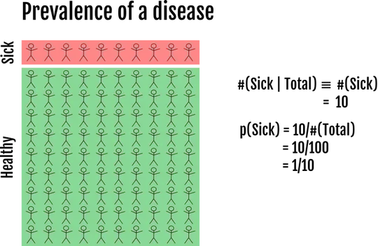
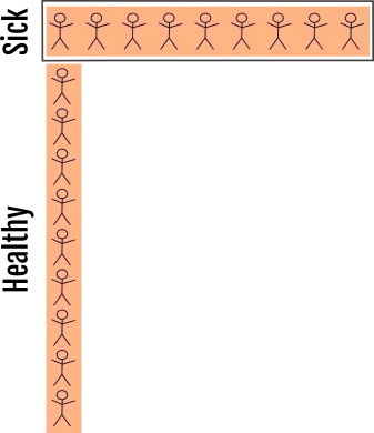
Let’s use the following example, where 1 in 10 people are sick. We denote [sic] could write p(Sick | Total population) = the probability of being sick given that you study the whole population = 0.1. But in the case when you study the whole population you just write p(Sick).

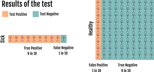
To simplify the example we assume that we know which ones are sick and which ones are healthy, but in a real test you don’t know that information. Now we test everybody for the disease:

The number of positive results among the sick population (#(Positive | Sick) is 9. These people are the true positives, a value that it’s known for tests:

#(Positive | Sick) = 9
p(Positive | Sick) = 9/#(Sick) = 9/10 = True Positive Rate

Now the interesting question, what is the probability of being sick if you test positive? (in math: p(Sick | Positive))

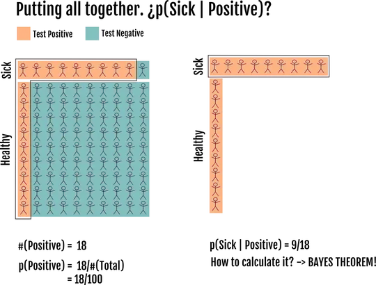
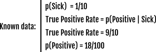
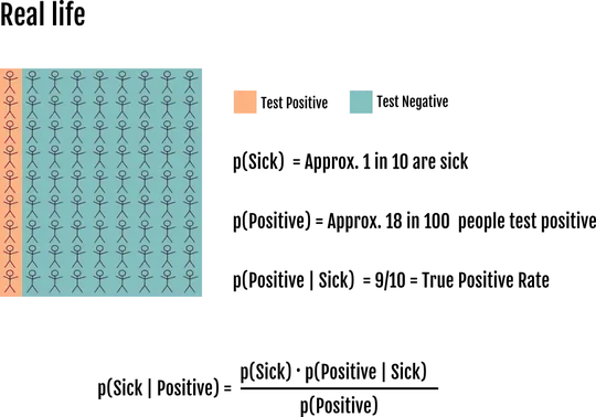
In the figure above we have all the information, and therefore we can count the sick people among the positive results to say that the probability of being sick if you tested positive is 9/18 = 50%. However in real life you only know that 18/100 have tested positive. To know that 50% of those are false positives you can use the Bayes Theorem. But we will derive it here. All the information we know is:

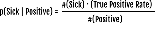
To remind you, we want to calculate the people inside the square #(Sick | Positive).

The intuition is that if we know that there are 10 sick people (#(Sick)) and the true positive rate is 0.9, then #(Sick | Positive) = 9.

In math:

For the probability we divide among the studied population (the positive results) to get:

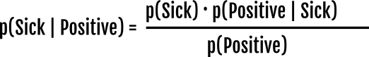
But we don’t know exactly how many people are sick, only the probability, so we can divide both parts of the fraction by the #(Total) and get probabilities of being sick and of testing positive.

And you have successfully derived the Bayes Theorem!

To recap:

Answer 4

A physical argument to explain it was very clearly depicted by Galton in a two stage quincunx in the late 1800,s.

See figure 5 in Stigler, Stephen M. 2010. Darwin, Galton and the statistical enlightenment. Journal of the Royal Statistical Society: Series A 173(3):469-482.

I have a rudimentary animation of it here (requires adequate pdf support to run).

I have also turned it into an allegory about an orange falling on Galton's head which I will try to upload in the future.

Or perhaps you might prefer the ABC rejection picture here.

An exercise based on it is here.