22

I have a GLMM with a binomial distribution and a logit link function and I have the feeling that an important aspect of the data is not well represented in the model.

To test this, I would like to know whether or not the data is well described by a linear function on the logit scale. Hence, I would like to know whether the residuals are well-behaved. However, I can not find out at which residuals plot to plot and how to interpret the plot.

Note that I am using the new version of lme4 (the development version from GitHub):

packageVersion("lme4")
## [1] ‘1.1.0’

My question is: How do I inspect and interpret the residuals of a binomial generalized linear mixed models with a logit link function?

The following data represents only 17% of my real data, but fitting already takes around 30 seconds on my machine, so I leave it like this:

require(lme4)
options(contrasts=c('contr.sum', 'contr.poly'))

dat <- read.table("http://pastebin.com/raw.php?i=vRy66Bif")
dat$V1 <- factor(dat$V1)

m1 <- glmer(true ~ distance*(consequent+direction+dist)^2 + (direction+dist|V1), dat, family = binomial)

The simplest plot (?plot.merMod) produces the following:

plot(m1)

enter image description here

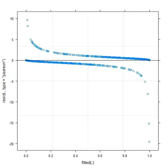
Does this already tell me something?

Henrik
  • 13,314
  • 9
  • 63
  • 123
  • 2
    I *might* find time to come back and take a crack at this, but I think the *general* answer is that it's hard to do a great deal with the residuals from binary models. My main discovery so far from zooming in on a bit on the plot you have above, and adding a smoothed line (using `type=c("p","smooth")` in `plot.merMod`, or moving to `ggplot` if you want confidence intervals) is that it looks like there's a small but significant pattern, which you might be able to fix by adopting a different link function. That's it so far ... – Ben Bolker Oct 02 '13 at 15:00
  • @BenBolker Thanks. And can you not just post this and the link to freakonomics as a response to the question? Then at least you would get the 150 points. – Henrik Oct 02 '13 at 15:32
  • 3
    I found this CV thread, http://stats.stackexchange.com/questions/63566/unexpected-residuals-plot-of-mixed-linear-model-using-lmer-lme4-package-in-r, to be very helpful. The post explains how to create a binned residuals plot in R. – Nova Aug 18 '14 at 20:09
  • @Henrik Would you please explain me how does the model `true ~ distance*(consequent+direction+dist)^2 + (direction+dist|V1)` work ? Will the model give estimate of interaction between `distance*consequent` , `distance*direction` , `distance*dist` and slope of `direction` and `dist` that varies with `V1` ? What does the square in `(consequent+direction+dist)^2` denote ? – ABC Jul 20 '15 at 10:48
  • @Henrik I ran your code and it shows the `Warning message: In checkConv(attr(opt, "derivs"), opt$par, ctrl = control$checkConv, : Model failed to converge with max|grad| = 0.123941 (tol = 0.001, component 1)` . Why ? – ABC Jul 20 '15 at 10:49
  • You may also want to have a look at the new DHARMa R package, which uses simulations from the fitted model to transform the residuals back to a standardized space, see examples in https://cran.r-project.org/web/packages/DHARMa/vignettes/DHARMa.html – Florian Hartig Jan 11 '17 at 22:33

5 Answers5

21

Short answer since I don't have time for better: this is a challenging problem; binary data almost always requires some kind of binning or smoothing to assess goodness of fit. It was somewhat helpful to use fortify.lmerMod (from lme4, experimental) in conjunction with ggplot2 and particularly geom_smooth() to draw essentially the same residual-vs-fitted plot you have above, but with confidence intervals (I also narrowed the y limits a bit to zoom in on the (-5,5) region). That suggested some systematic variation that could be improved by tweaking the link function. (I also tried plotting residuals against the other predictors, but it wasn't too useful.)

I tried fitting the model with all 3-way interactions, but it wasn't much of an improvement either in deviance or in the shape of the smoothed residual curve.

Then I used this bit of brute force to try inverse-link functions of the form $(\mbox{logistic}(x))^\lambda$, for $\lambda$ ranging from 0.5 to 2.0:

## uses (fragile) internal C calls for speed; could use plogis(),
##  qlogis() for readability and stability instead
logitpower <- function(lambda) {
    L <- list(linkfun=function(mu)
              .Call(stats:::C_logit_link,mu^(1/lambda),PACKAGE="stats"),
              linkinv=function(eta)
              .Call(stats:::C_logit_linkinv,eta,PACKAGE="stats")^lambda,
              mu.eta=function(eta) {
                  mu <-  .Call(stats:::C_logit_linkinv,eta,PACKAGE="stats")
                  mu.eta <-  .Call(stats:::C_logit_mu_eta,eta,PACKAGE="stats")
                  lambda*mu^(lambda-1)*mu.eta
              },
              valideta = function(eta) TRUE ,
              name=paste0("logit-power(",lambda,")"))
    class(L) <- "link-glm"
    L
}

I found that a $\lambda$ of 0.75 was slightly better than the original model, although not significantly so -- I may have been overinterpreting the data.

See also: http://freakonometrics.hypotheses.org/8210

Ben Bolker
  • 34,308
  • 2
  • 93
  • 126
4

You can plot the residuals against the predictors using simulation techniques in DHARMa package, it also offers a range of diagnostics such as overdispersion, and outliers, I think its a practical and simple assessment tool for GLMM. Check it out: https://cran.r-project.org/web/packages/DHARMa/vignettes/DHARMa.html

AhmadMkhatib
  • 106
  • 4
4

This is very common theme on biostatistics/epidemiology courses, and there are not very good solutions for it, basically due to the nature of the model. Often the solution has been to avoid detailed diagnostics using the residuals.

Ben already wrote that diagnostics often require either binning or smoothing. Binning of residuals is (or was) available in the R package arm, see e.g., this thread. In addition, there are some work done that uses predicted probabilities; one possibility is the separation plot that has been discussed earlier in this thread. Those might or might not directly help in your case, but could possible help the interpretation.

JTT
  • 1,295
  • 9
  • 13
-1

You could use AIC instead of residual plots to check fit of model. Command in R: AIC(model1) it will give you a number...so then you need to compare this with another model (with more predictors, for example) -- AIC(model2), which will yield another number. Compare the two outputs, and you'll want the model with the lower AIC value.

By the way, things like AIC and log likelihood ratio are already listed when you get the summary of your glmer model, and both will give you useful info on fit of model. You want a large negative number for log likelihood ratio to reject the null hypothesis.

  • 4
    This would be more useful if OP was trying to compare competing models, but it doesn't seem like that's what they're trying to do, and AIC cannot be used to evaluate absolute model fit. – Patrick Coulombe Mar 18 '16 at 01:04
-4

Fitted vs residuals plot should not show any (clear) pattern. The plot shows that the model does not work well with the data. See http://www.r-bloggers.com/model-validation-interpreting-residual-plots/