I'm not an expert in statistics as well, but I recently read the excellent book by Efron/Tibshirani (1997) and the bootstrap is a quite capable tool of questions such as yours. As pointed out here in the excellent answer by cardinal, the bootstrap really doesn't need specific assumptions, but performs very well quite generally.
With respect to your problem, this means that it can help to just run a bootstrap. I'm gonna do this here in R:
#Load required packages
library(boot)
library(MASS) #To simulate multivariate normally distributed observations
set.seed(369)
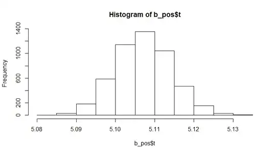
#Run bootstrap in the case of a positive correlation between x and y
N <- 1e4
X <- mvrnorm(N, mu=c(100,20),
Sigma = diag(c(20,5)) %*% matrix(c(1,0.9,0.9,1), nrow=2) %*% diag(c(20, 5)))
r <- X[,1]/X[,2]
b_pos <- boot(data=r,
statistic=function(x, i) mean(x[i]),
R=5000)
hist(b_pos$t)
#Run bootstrap in the case of a negative correlation between x and y
X <- mvrnorm(N, mu=c(100,20),
             Sigma = diag(c(20,5)) %*% matrix(c(1,-0.95,-0.95,1), nrow=2) %*% diag(c(20, 5)))
r <- X[,1]/X[,2]

b_neg <- boot(data=r,
          statistic=function(x, i) mean(x[i]),
          R=5000)
hist(b_neg$t)
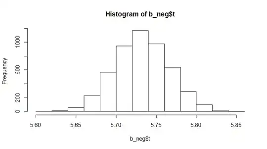
So what I find interesting here is the fact that the distribution seems to be shifted to the right with a decreasing correlation between $x$ and $y$. However, the mean always seems to be above $E[x]/E[y]$ which would be 5 in this case. (Note that $x$/$y$ is normally distributed with mean 100/20 and standard deviation of 20/5 here. I'm pretty sure that this result can be derived analytically quite easily for a trained statistician, but that's the beauty of the bootstrap: Even people without that background knowledge can get a fast feeling for the distribution of any statistic (and even trained statistician are often unable to derive distributional forms because there simply doesn't exist an analytical solution).
Now it's also easy to adjust the example to find out how $E[x]/E[y]$ behaves:
b_alt <- boot(data=X,
              statistic=function(x, i) mean(X[i, 1])/mean(X[i,2]),
              R=5000)
hist(b_alt$t)
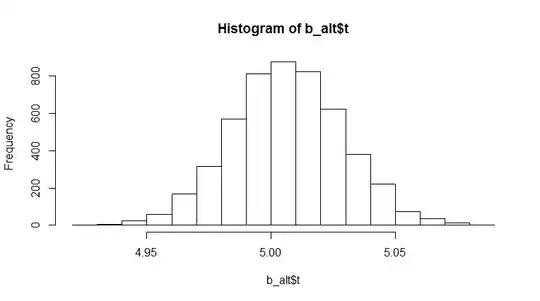
This is just centered around 100/20=5 as expected. Note, however, that things change quite dramatically if you center both variables around 0. Then, $E[x]/E[y]$ is not well-behaved anymore because the the denominator end up very close to zero quite often, whereby $E[x/y]$ first calculates the ratios and then averages, which averages the outliers.