30

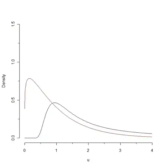
Look at this picture: enter image description here

If we draw a sample from the red density then some values are expected to be less than 0.25 whereas it is impossible to generate such a sample from the blue distribution. As a consequence, the Kullback-Leibler distance from the red density to the blue density is infinity. However, the two curves are not that distinct, in some "natural sense".

Here is my question: Does it exist an adaptation of the Kullback-Leibler distance that would allow a finite distance between these two curves?

kjetil b halvorsen
  • 63,378
  • 26
  • 142
  • 467
ocram
  • 19,898
  • 5
  • 76
  • 77
  • 1
    In what "natural sense" are these curves "not that distinct"? How is this intuitive closeness related to any statistical property? (I can think of several answers but am wondering what you have in mind.) – whuber Feb 05 '11 at 15:57
  • 1
    Well... they are pretty close to each other in the sense that both are defined on positive values; they both increase and then decrease; both have actually the same expectation; and the Kullback Leibler distance is "small" if we restrict to a portion of the x-axis... But in order to link these intuitive notions to any statistical property, I would need some rigourous definition for these features... – ocram Feb 05 '11 at 17:47
  • https://en.wikipedia.org/wiki/Statistical_distance – Memming Aug 14 '15 at 17:13

4 Answers4

21

You might look at Chapter 3 of Devroye, Gyorfi, and Lugosi, A Probabilistic Theory of Pattern Recognition, Springer, 1996. See, in particular, the section on $f$-divergences.

$f$-Divergences can be viewed as a generalization of Kullback--Leibler (or, alternatively, KL can be viewed as a special case of an $f$-Divergence).

The general form is $$ D_f(p, q) = \int q(x) f\left(\frac{p(x)}{q(x)}\right) \, \lambda(dx) , $$

where $\lambda$ is a measure that dominates the measures associated with $p$ and $q$ and $f(\cdot)$ is a convex function satisfying $f(1) = 0$. (If $p(x)$ and $q(x)$ are densities with respect to Lebesgue measure, just substitute the notation $dx$ for $\lambda(dx)$ and you're good to go.)

We recover KL by taking $f(x) = x \log x$. We can get the Hellinger difference via $f(x) = (1 - \sqrt{x})^2$ and we get the total-variation or $L_1$ distance by taking $f(x) = \frac{1}{2} |x - 1|$. The latter gives

$$ D_{\mathrm{TV}}(p, q) = \frac{1}{2} \int |p(x) - q(x)| \, dx $$

Note that this last one at least gives you a finite answer.

In another little book entitled Density Estimation: The $L_1$ View, Devroye argues strongly for the use of this latter distance due to its many nice invariance properties (among others). This latter book is probably a little harder to get a hold of than the former and, as the title suggests, a bit more specialized.


Addendum: Via this question, I became aware that it appears that the measure that @Didier proposes is (up to a constant) known as the Jensen-Shannon Divergence. If you follow the link to the answer provided in that question, you'll see that it turns out that the square-root of this quantity is actually a metric and was previously recognized in the literature to be a special case of an $f$-divergence. I found it interesting that we seem to have collectively "reinvented" the wheel (rather quickly) via the discussion of this question. The interpretation I gave to it in the comment below @Didier's response was also previously recognized. All around, kind of neat, actually.
cardinal
  • 24,973
  • 8
  • 94
  • 128
  • 1
    Very nice! I am going to try to find "A Probabilistic Theory of Pattern Recognition" and to understand its chapter 3! – ocram Feb 06 '11 at 08:11
  • 1
    good answer, note that most often $D_{TV}$ is defined another way which makes it half the $L_1$ distance. – robin girard Feb 17 '11 at 10:52
  • 1
    @robin, thanks for your comment. Yes, I realize this. I was just trying to avoid a messy extraneous constant in the exposition. But, strictly speaking, you're correct. I've updated it accordingly. – cardinal Feb 18 '11 at 13:33
  • 3
    Your addendum is the most useful piece of information I ran into on stats.SE, so far. All my warmest thanks for this. I simply reproduce here the reference you gave: http://research-repository.st-andrews.ac.uk/bitstream/10023/1591/1/Endres2003-IEEETransInfTheory49-NewMetric.pdf Endres and Schindelin, A new metric for probability distributions, *IEEE Trans. on Info. Thy.*, vol. 49, no. 3, Jul. 2003, pp. 1858-1860. – Did Feb 28 '11 at 12:07
  • 1
    @Didier, well, it was more a happy accident than anything else. No one was responding to the other question, so I decided to try to figure out what the Jensen-Shannon Divergence was in the first place. Once I found the definition, it seemed reasonable to connect the two questions via my addendum. I'm glad you found it useful. Regards. – cardinal Mar 01 '11 at 03:38
20

The Kullback-Leibler divergence $\kappa(P|Q)$ of $P$ with respect to $Q$ is infinite when $P$ is not absolutely continuous with respect to $Q$, that is, when there exists a measurable set $A$ such that $Q(A)=0$ and $P(A)\ne0$. Furthermore the KL divergence is not symmetric, in the sense that in general $\kappa(P\mid Q)\ne\kappa(Q\mid P)$. Recall that $$ \kappa(P\mid Q)=\int P\log\left(\frac{P}{Q}\right). $$ A way out of both these drawbacks, still based on KL divergence, is to introduce the midpoint $$R=\tfrac12(P+Q). $$ Thus $R$ is a probability measure, and $P$ and $Q$ are always absolutely continuous with respect to $R$. Hence one can consider a "distance" between $P$ and $Q$, still based on KL divergence but using $R$, defined as $$ \eta(P,Q)=\kappa(P\mid R)+\kappa(Q\mid R). $$ Then $\eta(P,Q)$ is nonnegative and finite for every $P$ and $Q$, $\eta$ is symmetric in the sense that $\eta(P,Q)=\eta(Q,P)$ for every $P$ and $Q$, and $\eta(P,Q)=0$ iff $P=Q$.

An equivalent formulation is $$ \eta(P,Q)=2\log(2)+\int \left(P\log(P)+Q\log(Q)-(P+Q)\log(P+Q)\right). $$

Addendum 1 The introduction of the midpoint of $P$ and $Q$ is not arbitrary in the sense that $$ \eta(P,Q)=\min [\kappa(P\mid \cdot)+\kappa(Q\mid \cdot)], $$ where the minimum is over the set of probability measures.

Addendum 2 @cardinal remarks that $\eta$ is also an $f$-divergence, for the convex function $$ f(x)=x\log(x)−(1+x)\log(1+x)+(1+x)\log(2). $$

Did
  • 1,577
  • 14
  • 23
  • 2
    @Marco, @Didier Piau, it might be noted that @Didier's suggestion is another special case of an $f$-divergence where $f(x) = x \log x - (1+x) \log( \frac{1+x}{2} )$. – cardinal Feb 06 '11 at 17:26
  • 1
    @Marco, @Didier Piau, an alternative formulation which has some evocative nature is $\eta(P, Q) = \int P \log P + \int Q \log Q - 2 \int R \log R = 2 H(R) - (H(P) + H(Q))$ and so $\eta(P,Q) = 2 ( H(\mu(P,Q)) - \mu(H(P), H(Q))$ where $\mu(x,y) = \frac{x+y}{2}$. In other words, $\frac{1}{2} \eta(P,Q)$ is "difference between the entropy of the average measure and the average entropy of the measures". – cardinal Feb 06 '11 at 17:30
  • 3
    Isn't this just the Jensen-Shannon divergence? – Memming Jul 28 '13 at 13:36
  • [Seems to be](https://en.wikipedia.org/wiki/Jensen%E2%80%93Shannon_divergence). – Did Jul 29 '13 at 09:59
10

The Kolmogorov distance between two distributions $P$ and $Q$ is the sup norm of their CDFs. (This is the largest vertical discrepancy between the two graphs of the CDFs.) It is used in distributional testing where $P$ is an hypothesized distribution and $Q$ is the empirical distribution function of a dataset.

It is hard to characterize this as an "adaptation" of the KL distance, but it does meet the other requirements of being "natural" and finite.

Incidentally, because the KL divergence is not a true "distance," we don't have to worry about preserving all the axiomatic properties of a distance. We can maintain the non-negativity property while making the values finite by applying any monotonic transformation $\mathbb{R_+} \to [0,C]$ for some finite value $C$. The inverse tangent will do fine, for instance.

whuber
  • 281,159
  • 54
  • 637
  • 1,101
  • 1
    Thank you for your suggestion about the Kolmogorov distance. Can you make your comment about the monotonic transformation a little bit more explicit? Thx – ocram Feb 06 '11 at 08:13
  • 1
    @Marco I don't understand how one could be any more explicit. Do you mean restating what I wrote in terms of a formula such as $\arctan(KL(P,Q))$ or $f(KL(P,Q))$ for $f:\mathbb{R_+} \to [0,C]$ with $x \ge y$ implies $f(x) \ge f(y)$ for all $x,y \ge 0$? – whuber Feb 06 '11 at 19:12
  • 1
    Yes, that's what I meant :-) I was not sure on what to apply the transformation. Now, it is clear, thx – ocram Feb 07 '11 at 07:17
  • 1
    @Marco: I am lost. Do you settle for the Kolmogorov distance (which is always finite but has nothing in common with KL divergence)? Or for a bounded monotone transform of KL divergence (such as $\arctan$)? In the example of your post (and in any other *not absolutely continuous* example), the latter produces the supremum of the transform ($\pi/2$ if you settle for $\arctan$). In effect, this abandons any idea of estimating a *distance* between such probability measures more precisely than saying they are *far far away* (whether you encode this by $\pi/2$ or by $+\infty$ is irrelevant). – Did Feb 07 '11 at 08:47
  • @Didier Yes, the transformed KL divergence (when symmetrized, as you describe) might not satisfy the triangle inequality and therefore would not be a distance, but it would still define a topology (which would likely be metrizable). You would thereby give up little or nothing. I remain agnostic about the merits of doing any of this: it seems to me this is just a way of papering over the difficulties associated with infinite values of the KL divergence in the first place. – whuber Feb 07 '11 at 13:22
  • @whuber Topology and the (defect of) triangle inequality are not my point here. I simply wondered why Marco suddenly seemed happy with the $\arctan$ artefact you suggested, although this artefact leaves every pair of not absolutely continuous probability measures as infinitely *far far away* from each other as they were with respect to KL divergence. Note also that $\eta$ is not only (and not mainly) a *symmetrized* version of KL, more importantly $\eta$ is *finitized*. .../... – Did Feb 07 '11 at 13:52
  • .../... Example: for every $t>0$, let $P_t$ denote the uniform probability distribution on the interval $(0,t)$. For every $t\ne s$, $P_t$ and $P_s$ are at infinite distance for KL but $\eta(P_t,P_s)$ is positive and finite and depends non trivially on $(t,s)$. Inter alia, $\eta$ *quantifies* the fact that, if $t – Did Feb 07 '11 at 13:53
  • @Didier Could you clarify what you mean by "finitized"? After all, two distributions can be infinitely far apart w.r.t. $\eta$, even when their supports overlap. The family of uniforms you discuss is special in that in each pair, one of them is absolutely continuous w.r.t the other. (Even that doesn't in general guarantee $\eta$ is finite, but it suffices in this case.) However, we are moving off onto a tangential topic here: what we are missing is any sense of *why* there is a concern about the possibility of an infinite divergence (or infinite distance). – whuber Feb 07 '11 at 13:58
  • @whuber Why is there a concern about the possibility of infinite distance? Dunno... maybe because infinite distances is the feature the OP asked a remedy for in the first place... Re $\eta$, let me stress once again that $\eta(P,Q)$ is finite for **every** probability measures $P$ and $Q$. – Did Feb 07 '11 at 14:09
  • @whuber Here is another example to let you better understand the behaviour of $\eta$. Let $U_t$ denote the uniform distribution on the interval $(t,1+t)$. Then $\eta(U_t,U_s)=\min(1,|t-s|)2\log(2)$. No $U_t$ and $U_s$ are absolutely continuous with respect to each other unless $s=t$. Finally, note that $\eta\le2\log(2)$ uniformly, and that $\eta(P,Q)=2\log(2)$ iff $P$ and $Q$ are mutually singular. – Did Feb 07 '11 at 14:23
  • @Didier Thank you: I misread the formula for $\eta$ until just this moment; I had confused it with the $\delta$ defined in another answer. Too hasty. I appreciate your patient explanations as well as the clarifications provided by @cardinal in comments to your answer. – whuber Feb 07 '11 at 14:59
2

Yes there does, Bernardo and Reuda defined something called the "intrinsic discrepancy" which for all purposes is a "symmetrised" version of the KL-divergence. Taking the KL divergence from $P$ to $Q$ to be $\kappa(P \mid Q)$ The intrinsic discrepancy is given by:

$$\delta(P,Q)\equiv \min \big[\kappa(P \mid Q),\kappa(Q \mid P)\big]$$

Searching intrinsic discrepancy (or bayesian reference criterion) will give you some articles on this measure.

In your case, you would just take the KL-divergence which is finite.

Another alternative measure to KL is Hellinger distance

EDIT: clarification, some comments raised suggested that the intrinsic discrepancy will not be finite when one density 0 when the other is not. This is not true if the operation of evaluating the zero density is carried out as a limit $Q\rightarrow 0$ or $P\rightarrow 0$ . The limit is well defined, and it is equal to $0$ for one of the KL divergences, while the other one will diverge. To see this note:

$$\delta(P,Q)\equiv \min \Big[\int P \,\log \big(\frac{P}{Q}\big),\int Q \log \big(\frac{Q}{P}\big)\Big]$$

Taking limit as $P\rightarrow 0$ over a region of the integral, the second integral diverges, and the first integral converges to $0$ over this region (assuming the conditions are such that one can interchange limits and integration). This is because $\lim_{z\rightarrow 0} z \log(z) =0$. Because of the symmetry in $P$ and $Q$ the result also holds for $Q$.

cardinal
  • 24,973
  • 8
  • 94
  • 128
probabilityislogic
  • 22,555
  • 4
  • 76
  • 97
  • 1
    Even the "intrinsic discrepancy" will be infinite when $P$ is zero with positive probability for $Q$ and *vice versa,* even if $P$ and $Q$ are otherwise identical. – whuber Feb 05 '11 at 15:56
  • 1
    Yes... I am afraid that the intrinsic discrepancy does not fulfil the requirement. But thank you for the suggestion. Any other suggestion would be appreciated. – ocram Feb 05 '11 at 17:49
  • 1
    It does fulfil the requirement, if you restrict the support of the blue density to be where it has strictly positive support, just as you have for the red one (>0) – probabilityislogic Feb 05 '11 at 22:01
  • Yes indeed, restricting the support is the simplest idea but I guess that the resulting KL distance should be reduced in some way in order to take that trick into account... – ocram Feb 06 '11 at 08:10
  • Actually now that I think of it, you don't need to restrict the support, because the $0$ in the log gets canceled out by the $0$ in the pdf multiplying it. So you actually get $Lim_{P\rightarrow 0} P log(\frac{P}{Q})= Lim_{P\rightarrow 0} P log(P)=0$, and the intrinsic discrepancy is defined after all! – probabilityislogic Feb 06 '11 at 14:19
  • 3
    @probabilityislogic: I do not unerstand your last remarks. First, let us give their proper names to the notions involved and say that $P$ is absolutely continuous with respect to $Q$ (denoted $P\ll Q$) if, for every measurable $A$, $Q(A)=0$ implies $P(A)=0$. Now, notwithstanding your somewhat mysterious (to me) limit considerations, your $\delta(P,Q)$ is finite iff $P\ll Q$ or $Q\ll P$. .../... – Did Feb 06 '11 at 15:25
  • 2
    .../... A way out of the conundrum you seem to be dug into might be to introduce the mid-point measure $P+Q$. Since $P\ll P+Q$ and $Q\ll P+Q$, the quantity $\eta(P,Q):=\kappa(P|P+Q)+\kappa(Q|P+Q)$ is always finite. Furthermore $\eta(P,Q)=0$ iff $P=Q$ and $\eta$ is symmetric. Hence $\eta(P,Q)$ indeed measures a kind of "distance" between $P$ and $Q$. – Did Feb 06 '11 at 15:26
  • Edit: the midpoint is $\frac12(P+Q)$ and $\eta(P,Q):=\kappa(P|P+Q)+\kappa(Q|P+Q)+2\log2$. – Did Feb 06 '11 at 15:33
  • @probabilityislogic, @Didier Piau, A simple example to show what Didier is saying is to take $p(x) = 1_{(x \in (0,1))}$ and $q(x) = 1_{(x \in (1,2))}$. Then $\delta(p,q)$ is infinite. If you want a more extreme example, for any $\epsilon > 0$, let $q(x) \equiv q_{\epsilon}(x) = 1_{(x \in (\epsilon, 1+\epsilon))}$. – cardinal Feb 06 '11 at 15:43
  • @cardinal: Indeed. I now wrote an answer to the OP explaining this "midpoint+KL" stuff. – Did Feb 06 '11 at 15:50
  • @probabilityislogic, A simple example which I believe shows where your limiting argument fails is to consider $p(x) = 1_{(x \in (0,1/2)\cap\mathbf{Q})} + 2 1_{(x \in (1/2,1))}$. Then $p(x)$ is zero on a subset of $(0,1/2)$ with positive measure, but $p(x) \not\to 0$ for any $x \in (0,1/2)$. So your limit argument needs further conditions, even if it were to otherwise work. A sort of work-around is not to focus on the limits of $p$, but instead to define $x \log x$ on $[0,\infty]$ via an extension by continuity. The other problems with your development would still remain, however. – cardinal Feb 06 '11 at 15:50
  • @cardinal - in the example you give, the distance *should* be infinite, because the supports are *disjoint* (and thus not comparable). – probabilityislogic Feb 08 '11 at 06:55
  • @cardinal: I think the measure I made requires one measure to have a support of a subset of the other. If there is a "zero" region in P, and not Q, and also a "zero" region in Q, and not in P, then it is infinite. If the supports are nested, then it is always finite – probabilityislogic Feb 08 '11 at 07:33
  • @probabilityislogic, the second remark you make is essentially the concept of absolute continuity that @Didier was bringing to your attention. As regards your first comment, look again. I gave you the "extreme" example for a very good reason: the difference in support can be made *arbitrarily* small and yet your measure $\delta$ remains infinite. – cardinal Feb 08 '11 at 12:52
  • @cardinal - I take your point, but my answer does apply reasonably well to the particular densities being compared, as the supports are nested in this case. – probabilityislogic Feb 09 '11 at 13:15
  • @probabilityaslogic, I guess I viewed the exercise as an attempt to find a good distance measure in a general setting. If the objective is to find a good measure that matches one's intuition for a single particular example, you might as well pick your favorite number and assign that value to be the distance. – cardinal Feb 09 '11 at 13:31