Generating non-homogeneous spatial Gaussian data

Question

I want to generate a spatial data following multivariate Gaussian distribution.

However, I don't want it to be homogeneous, meaning I don't want the correlation/covariance to be homogeneous. I want it to be heterogeneous.

Any suggestions on how to generate such data?

Here is an example of what I mean by heterogeneous covariance matrix

   25.8621   25.1207   24.6305   24.3867
   25.1207   25.3719   24.8768   24.6305
   24.6305   24.8768   25.3719   25.1207
   24.3867   24.6305   25.1207   25.8621

There are four variables. As you can see the marginal variance is different which means C(0) is dependent on location. So does C(h) for any h. This is one method of generating heterogeneous data.

But I want some spatial data consisting of like land, lakes which have very less covariance between each other.

Sure, there are plenty of ways. It's important to specify more precisely what you mean by "multivariate gaussian" and non "homogeneous." After all, you can take any finite number of locations and generate multivariate gaussian values according to any positive semidefinite covariance matrix associated with those locations. Ultimately this kind of construction, by its very generality, is not very useful: what is your *real* question? Why do you need to generate such data? — whuber, Aug 02 '13 at 02:16
@whuber. Actually, my data is spatial and the variables in each location form a multivariate gaussian distribution. Normally, when I specify the correlation lets say, then I am assuming that it is homogeneous meaning it behaves the same everywhere. However, I want to make it heterogeneous meaning different blocks in the spatial data could have different correlation function so it's not consistent with distance — user31820, Aug 02 '13 at 11:15
It is hard to tell whether you are talking about *heteroscedastic* variables, which may have different covariance matrices at different locations, or a *non-stationary* field, where the covariance matrix relates variables at one location to those at another location, or both. Could you please clarify this? — whuber, Aug 02 '13 at 13:52
Then what is the matter with stipulating separate covariance matrices for each of your spatial locations and generating data independently from those distributions? — whuber, Aug 03 '13 at 18:40
@whuber. I can do that. But that will give me sharp discontinuity. Lets say I divide the region into four draw from a different covariance/correlation function/matrix. It will give me four totally discontinuous regions. I want somewhat smoother transition not totally discontinuous. Lets say I have two separate regions. For one I will draw samples from gaussian with mean 0, other with mean 10,further use different correlation structure. Definitely the values will be different. But I want somewhat smoother transition — user31820, Aug 04 '13 at 05:45
@whuber. What I want is kind of a partition. Suppose I have land followed by a lake followed by the land itself. What I want is the variables in the land are correlated more with the variables of the land but less with that of lake and the variables of the lake with the variables of the lake itself. How can I generate such data. So I want some kind of discontinuity — user31820, Aug 04 '13 at 13:06
Are those your only criteria? Or are you trying to reproduce the characteristics of actual data? — whuber, Aug 05 '13 at 00:45
@whuber. Yeah they are my criteria. I want a heterogeneous spatial gaussian field. Lets say an area/land with a lake in between two pieces of land and I am measuring a field. All the locations in the land they have smooth covariance dropping at the lake suddenly. Similarly the location in the lakes have smooth covariance with the locations in the lake and dropping suddenly with the locations in the land. Let say Two pieces by land divided by a lake. I want to simulate some synthetic data with that criteria. I can try tuning the sharpness of the discontinuity — user31820, Aug 05 '13 at 01:11
It's still unclear what you're looking for. For instance, you could independently generate data on land and on lakes: that would assure a vanishingly small covariance between land data and lake data. But what do you mean by "tune the sharpness"? I suspect you have some mental picture of what you want that you haven't fully or accurately expressed yet. — whuber, Aug 06 '13 at 14:43
@whuber. If I generate a covariance matrix for a grid of size 100x100 with different marginal variance and the covariances not being a function of distance only but location itself, then it is heterogeneous by itself isn't it? — user31820, Aug 08 '13 at 11:21
I'm afraid I don't understand adequately what you mean by "marginal variance" nor "heterogeneous," but if I interpret this as saying that when the covariance matrix is not invariant under translations of the data supports, then it must be a covariance matrix for a nonstationary process, then I can agree that you're right. — whuber, Aug 08 '13 at 16:30
@whuber. I have an example in my original question. I am assuming that nonstationary is equivalent to heterogeneous. I have read that stationary being equivalent to homogeneous. So I am assuming the opposite case as well — user31820, Aug 08 '13 at 16:47

EngrStudent · Answer 1 · 2013-08-10T14:53:22.913

You might find this useful: http://www.mathworks.com/help/stats/gmdistribution.fit.html

MU1 = [1 2];
SIGMA1 = [2 0; 0 .5];
MU2 = [-3 -5];
SIGMA2 = [1 0; 0 1];
X = [mvnrnd(MU1,SIGMA1,1000);mvnrnd(MU2,SIGMA2,1000)];

scatter(X(:,1),X(:,2),10,'.')
hold on
options = statset('Display','final');
obj = gmdistribution.fit(X,2,'Options',options);
h = ezcontour(@(x,y)pdf(obj,[x y]),[-8 6],[-8 6]);

Now these covariances are only diagonal. You can fix that by changing numbers.

The "gmdistribution.fit" is where you get the contour values.

So here is a plot that this would create: enter image description here

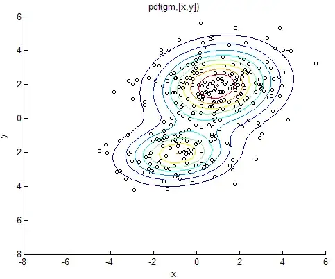
Now you can see that it creates two multivariate gaussian distributions. You only need to create one.

The function that generates the data is:

mvnrnd(MU1,SIGMA1,1000)

the mvnrnd, or mv-n-rnd is the multivariate normal random number generator. Its inputs are the multivariate mean, covariance matrix, and desired sample count. The output is an array of numbers of dimension informed by mu1.

The example covariance that you provided was 5 dimensional. Here is something "hackable" that you should be able to convert for your own non-nefarious purposes.

%this creates a 5-dimensional mean

MU1 = rand(1,5)+[1,2,3,4,5];

%this creates a 5x5 covariance, diagonally dominant

SIGMA1 = 23*rand(5,5)+eye(5);

%this is for consistent notation. previously it stacked multiple multivariate gaussians.

X = [mvnrnd(MU1,SIGMA1,1000)];

%this plots the dots

scatter(X(:,1),X(:,2),10,'.');

%this lets multiple plots overlay

hold on;

%this is a parm of the gm fit function. It says "display final result".

options = statset('Display','final');

%this fits a gaussian to the data

obj = gmdistribution.fit(X,1,'Options',options);

%this plots the contours of the fitted gaussian over the domain of the data

h = ezcontour(@(x,y)pdf(obj,[x y]),[min(X(:,1)) max(X(:,1))],...
                                   [min(X(:,2)) max(X(:,2))]);

Best of luck.

Some explanation would be welcome for those who do not care, or are unable, to run your code. What is it doing? What numbers must be changed to produce non-diagonal covariances? How exactly does your answer solve the problem? — whuber, Aug 09 '13 at 20:59
@whuber - that is how I often feel when I see R code. I will get to it later on (hopefully this evening) but I will try to annotate and describe. — EngrStudent, Aug 10 '13 at 00:45

Generating non-homogeneous spatial Gaussian data

1 Answers1