4

Say I have a data set composed of $N$ objects. Each object has a given number of measured values attached to it (three in this case):

$x_1[a_1, b_1, c_1], x_2[a_2, b_2, c_2], ..., x_N[a_N, b_N, c_N]$

meaning I have measured the properties $[a_i, b_i, c_i]$ for each $x$ object. The measurement space is thus the space determined by the variables $[a, b, c]$, where each $x$ object is represented by a point in it.

More graphically: I have $N$ objects scattered in a 3D space.

What I need is a way to determine the probability (or likelihood?, is there a difference?) of a new object $y[a_y, b_y, c_y]$ of belonging to this cloud of objects This probability calculated for any $x$ object will of course be very close to 1.

Is this feasible?


Add 1

To address AdamO's question: the object $y$ belongs to a set composed of $M$ mixed objects (with $M$ > $N$). This means that some objects in this set will have a high probability of belonging to the first data set ($N$) and others will have a lower probability. I'm actually interested in these low probability objects.

I can also come up with up to 3 more data sets of $N1$, $N2$, and $N3$ objects, all of them having the same global properties as those in the $N$ data set. Ie: an object in $M$ that has a low probability in $N$ will also have low probabilities when compared with $N1$, $N2$ and $N3$ (and viceversa: objects in $M$ of high probabilities of belonging to $N$ will also display high probabilities of belonging to $N1$, $N2$ and $N3$).


Add 2

According to the answer given in the question Interpretation/use of kernel density I can not derive the probability of a new object belonging to the set that generated the $kde/pdf$ (assuming I would even be able to resolve the equation for a non-unimodal $pdf$) because I have to make the a priori assumption that that new object was generated by the same process that generated the data set from which I obtained the $kde$. Could someone confirm this please?
Gabriel
  • 3,072
  • 1
  • 22
  • 49
  • Do you also have a random sample of objects that *don't* belong to the $x_i[a_i, b_i, c_i]$, $i \leq n$ group? – AdamO Jul 03 '13 at 19:17
  • @AdamO not exactly, please see expanded question. – Gabriel Jul 03 '13 at 19:36
  • so basically you're looking for a density based clustering algorithm? Do you have an expectation for how many clusters there ought to be, or is this completely unsupervised? – David Marx Jul 03 '13 at 20:47
  • 1
    The question in your Add2 is actually somewhat unrelated. The question has to do with the interpretation of the $y$ axis and whether it has a direct probability interpretation. That obviously is incorrect. However, integrating a KDE over distinct bounds *will* give you interpretable probability estimates. – AdamO Jul 07 '13 at 15:17
  • But the answer accepted mentions precisely the _area under the curve_ (ie: the integral of the $pdf$) and it still says it's not valid to interpret that as a probability of a point belonging to the set that generated that $pdf$. I think the last sentence pretty much says it all: _The kernel density estimate doesn't say anything about the probability a new value was generated by the same process._ What am I missing here? Thank you for your patience! – Gabriel Jul 07 '13 at 16:03

1 Answers1

2

The first question to address is: what's your distance metric? If you're comfortable with Euclidean space, by all means use that. However, you may want to transform these data onto an orthogonal basis using some kind of SVD and that can be done easily with any statistical software.

Given these data have been transformed into a suitable domain, you can estimate a probability density for these data using some kind of parametric or nonparametric estimation. Roughly normal data are adept to estimation via maximum likelihood, but density smoothers like the boxcar, or (better) a radial basis kernal smoother, will give you an estimate of the probability density ($\hat{f}$) over your domain ($\Omega$).

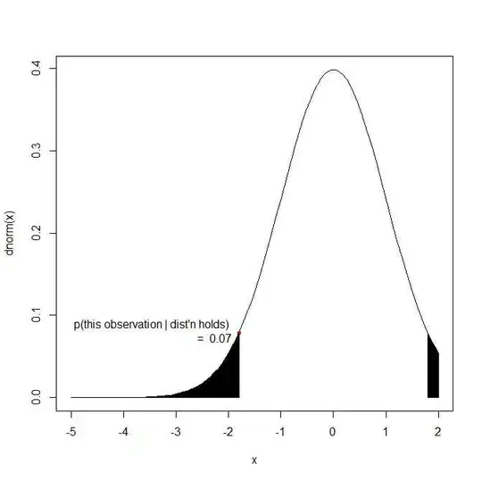
With these in place, we can evaluate a new observation in terms of its probability from having originated from that distribution. With a new observation taking values $x, y, z$, integrate the probability density over values of the support for which the density is less than the one you observed. This is well behaved for unimodal distributions. That is,

$$\mathcal{F}(x, y, z) = 1-\iiint_{r, s, t :\hat{f}(r, s, t) < \hat{f}(x, y, z)} \hat{f}(r,s,t)\,dr\,ds\,dt $$

This has a direct interpretation like a p-value (very roughly and blending Bayesian / Frequentist ideas): with this point, assuming it is generating from a known distribution (\hat{f}), what's the probability of observing another point as improbable or more improbable given it comes from this distribution? If this value is sufficiently small, we would rule that it is unlikely to have originated from the same distribution, though there is a chance that results in a Type I error.

curve(dnorm, from=-5, to=2)

points(x=-1.8, y=dnorm(-1.8), col='red', pch=20)

polygon(
  x=c(-5, seq(-5, -1.8, by=.1), -1.8),
  y=c(0, dnorm(seq(-5, -1.8, by=.1)), 0),
  col='black'
)

polygon(
  x=c(1.8, seq(1.8, 2, by=.1), 2),
  y=c(0, dnorm(seq(1.8, 2, by=.1)), 0),
  col='black'
)

text(-1.8, dnorm(-1.8), paste("p(this observation | dist'n holds) 
= ", round(pnorm(-1.8)*2, 2)), pos=2)

enter image description here

AdamO
  • 52,330
  • 5
  • 104
  • 209
  • I think I almost understand this answer (I have almost zero statistical training and what little I know is self-taught) So with this approach the hard part would be (assuming euclidean space is fine) obtaining the $\hat{f}$ probability density. Am I understanding correctly if I say that that $\hat{f}$ could be obtained through Duong's _kernel density estimator_ (http://www.jstatsoft.org/v21/i07)? – Gabriel Jul 03 '13 at 21:28
  • Yes, although Duong is hardly worth being the namesake for the method. Density estimation has been approached several times especially since the advent of statistical computing. – AdamO Jul 03 '13 at 21:47
  • I'm not sure I get how the integral should be performed. How do I set the limits of integration for a $\hat{f}$ in more than one dimensions where $\hat{f}$ behaves like this: http://imagebin.org/263440? – Gabriel Jul 04 '13 at 21:30
  • 3
    This solution appears to ignore all uncertainty in estimating $\hat{f}$ (which, for a kernel smoother, can be substantial). That changes the interpretation of the answer, which no longer can be viewed either as a probability nor as a p-value. How would you address this issue? – whuber Jul 05 '13 at 15:47
  • Was that last question directed at me or at AdamO whuber? I actually have no idea how to address the issue you point out (I wasn't even aware KDE's had big uncertainties associated to them). Would you say this answer is not correct? Do you have any ideas of how I could tackle this problem? – Gabriel Jul 05 '13 at 16:12
  • I've added some new info on the question that would point out to this answer not being correct. I'd really appreciate it if you could confirm this whuber. – Gabriel Jul 06 '13 at 01:55
  • 3
    @whuber +1 Yes, uncertainty in the estimate of the DF is a substantial caveat. For approximately Gaussian fields, estimating the joint density with ML would do substantially better. The question of "belonging to a set of objects" without the presence of a control or alternative comparison group is a question of consistency, i.e. how consistent is the observed point $y$ with the resampling prob dist-n of a fixed set of data. If $f$ were known, then the integral can be interpreted as a probability that a newly observed point having df $f$ belongs to any subset of $\Omega$ containing $y$ that... – AdamO Jul 07 '13 at 15:05
  • ... is *as* probable or *less* probable than any subset of $\Omega$ *not* containing $y$. – AdamO Jul 07 '13 at 15:06
  • @Gabriel I would estimate such an integral using either MCMC methods or direct numerical integration over a rough grid. – AdamO Jul 07 '13 at 15:12
  • @AdamO what I don't understand is how I would _set the limits of integration_ if the $pdf$ is not unimodal as the image I showed above. – Gabriel Jul 07 '13 at 23:22
  • The limits are defined by inverting the DF over ranges which are less than those at the observed DF at $y$. For instance, in my example, we observed $y = -1.8$ which has a standard normal density of 0.08. If I invert the normal DF to find which values have density less than 0.08, I get the $\Omega$ subsets $(-\infty, -1.8)$ and $(1.8, \infty)$ which have total probability area 0.07. – AdamO Jul 08 '13 at 16:32
  • Yes, that works for a _unimodal_ distribution but I have a 2D DF that behaves quite differently, please have a look here: http://stats.stackexchange.com/questions/63447/integrating-kernel-density-estimator-in-2d In this case obtaining those subsets is not straightforward and I don't understand if it could even be done. – Gabriel Jul 10 '13 at 11:26
  • It's quite straightforward actually. For smooth pdfs, you employ root finding algorithms (NR or `uniroot` in R) to find regions for which the PDF is *less* than $\hat{f}(Y)$ or *more* than $\hat{f}(Y)$, verify which sets are which, and then integrate. – AdamO Jul 10 '13 at 17:19
  • 1
    In 2D, you just need to parameterize connected curves in 2 space that determine lower and upper bounds. Think of an island and underwater regions on a map. – AdamO Jul 10 '13 at 17:50