3

I ran lm() (I'm using R, but I don't think anything else in this question is R specific) then realized I'd used the wrong input data, basically meaningless. Yet, I got a really good model:

Residuals:
      Min        1Q    Median        3Q       Max 
-0.069654 -0.003899 -0.000381  0.004722  0.083622 

Coefficients:
              Estimate Std. Error t value Pr(>|t|)    
(Intercept)  1.795e-02  1.800e-03   9.970   <2e-16 ***
x           -3.676e-06  3.848e-07  -9.554   <2e-16 ***
---

Residual standard error: 0.01416 on 11338 degrees of freedom
Multiple R-squared: 0.007986,   Adjusted R-squared: 0.007899 
F-statistic: 91.28 on 1 and 11338 DF,  p-value: < 2.2e-16 

I don't quite have permission to upload the data, and also it is large, but here is a plot of y and x (NB. x is on the vertical axis):

My real data

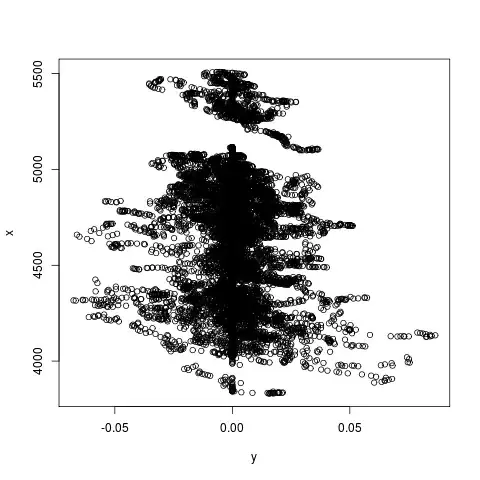
Okay, the break at roughly x==5200 is interesting, but basically it looks to me like for any value of x, y could be either side of y==0 with equal probability. So I don't see how it could possibly find a model with such a low p-value.

To help understand, I tried to do the same with random-looking data:

d=data.frame(
    y=(rnorm(10000,0,0.1))^2,
    x=5000+runif(10000)*500
    )
d$y=ifelse(runif(10000)<0.5,-d$y,d$y)

But lm(y~x,data=d) gives the terrible model I expected:

Residuals:
      Min        1Q    Median        3Q       Max 
-0.165179 -0.004537  0.000104  0.004742  0.134604 

Coefficients:
              Estimate Std. Error t value Pr(>|t|)
(Intercept)  1.439e-03  6.324e-03   0.228    0.820
x           -2.967e-07  1.203e-06  -0.247    0.805

Residual standard error: 0.01737 on 9998 degrees of freedom
Multiple R-squared: 6.082e-06,  Adjusted R-squared: -9.394e-05 
F-statistic: 0.06081 on 1 and 9998 DF,  p-value: 0.8052 

That random data looks like this:

random data

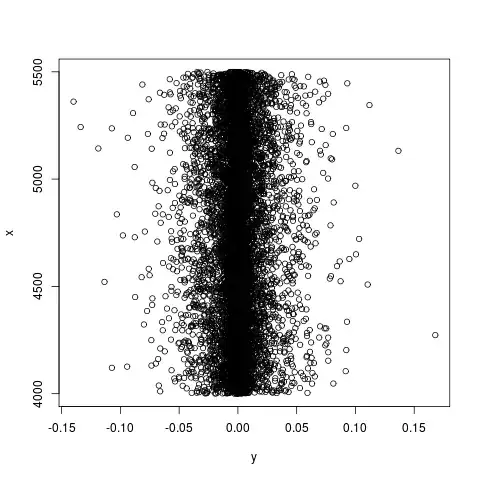
So, my real data and my random data behave completely differently when given to lm(), despite "x" looking equally useless as a predictor for "y" in both cases. It must be one of:

  • I'm misreading the linear model output
  • I'm asking the wrong question
  • The "x" in my real data is genuinely a good predictor for "y"
Darren Cook
  • 1,772
  • 1
  • 12
  • 26
  • Usually, x would be the horizontal axis and y the vertical axis on the graph. Looking at both graphs that way will perhaps make the differences more visible. – Gala May 07 '13 at 14:09
  • Related question: http://stats.stackexchange.com/q/5135/5503 – Darren Cook May 08 '13 at 00:17

1 Answers1

11

It is helpful to see the scatter plot and full display of results. But in my view there is really no surprise here once you look at all you have shown.

Multiple R-squared: 0.007986 does not to me imply a "really good model". (There could be a long debate on the limitations of that measure, but I don't think any of it weakens what is going on in your case.)

Your model is in effect y = constant + extremely slight trend with x. That constant is, roughly, the mean of y.

The residuals are all small, but so are all the values of y.

P-values that are very small are just side-effects of a very big sample size.

Looking at your scatter plots does underline that the underlying situations appear different, but fitting straight lines is not, in my view, going to illuminate either dataset.

[LATER] The very small but supposedly significant slope in the first case could be a side-effect of the small cluster of points in the bottom right of your plot. They are exerting just enough leverage to make a difference, I guess.

Another detail is that the intercept in the first case is significantly different from 0 at 1.795e-02. But that intercept estimate is, as usual, for x = 0, which is way outside the range of your x variable.

Nick Cox
  • 48,377
  • 8
  • 110
  • 156
  • +1. Incidentally, this also explains that the results have probably nothing to do with the apparent break around x=5200 – Gala May 07 '13 at 14:11
  • 1
    Large effects and large sample sizes both act to achieve small p-values. As was pointed out, the effect seems small (as pointed out, there is some structure in your first plot). However, your sample size is quite large. As a result, even a subtle pattern can be confidently distinguish from no pattern at all, i.e., significant. In the end there is a good reason why the p-value is small, but your example emphasizes why p-values are not the only criterion on which to judge a regression. – rbatt May 07 '13 at 16:26
  • Thanks. So I got seduced by the very low p-value, when I should have been looking at the low R² value! But, what exactly do a low p and low R² mean together? That it is very confident its suggested line captures 0.8% of the variance? Or that it is very confident it is not possible to capture more than 0.8% of the variance? Or something else? – Darren Cook May 07 '13 at 23:54
  • @rbatt (Your comment could've been an answer, I think). I wondered about this, but the random case is roughly the same sample size, and gives me a p-value of 0.8. So, the low p-value for the real data is saying there is genuine predictive ability in 'x'? (And then the low R² value adds: "but it doesn't help you much"?) – Darren Cook May 08 '13 at 00:00
  • 2
    Your example just underlines that very small effects can be significant with very large sample sizes, but here "significant" only means distinguishable statistically from zero. It's best not to talk in terms of anybody or anything being "confident". Also, R-square is only indirectly part of the formal inference. – Nick Cox May 08 '13 at 00:20
  • You might it helpful to put the scatter plots the right way up and then plot the regression lines on top. The slopes are both near zero, but one is 10x steeper than the other. Both nearly flat means low R-square in both cases, but the slope difference is enough to make a big difference to the P-value. – Nick Cox May 08 '13 at 00:35