Why my cdf of the convolution of n exponential distribution is not in the range(0,1)?

Question

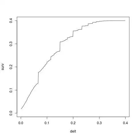
I assume that there are n exponential distribution that $x_i$ ~ $Exp(\lambda_i)$, i=1..n, and I want to calculate the cumulative distribution of $S=x_1+x_2+...+x_n$, the convolution of n exponential distribution. I used the formulation that I read in a paper given by, $$1-\sum_{i=1}^n (\prod \limits_{j=1,j\neq i}^n \frac{\lambda_j}{\lambda_j-\lambda_i})e^{-\lambda_i t}$$ but when I set $\lambda_i = 0.01i+2$, and $n=20$, then when t=0, the result is not equal to 0.

Answer 1

You can alternatively model this as an order distribution. There is a link between sums of exponentials and order distributions of exponentials.

Since you are looking for the special case of $\lambda_i = 0.01i+2$ and $n=20$ this link works. The sum is similar to the sampling of $m = 220$ exponential distributions with $\lambda = 0.01$ and taking the 20-th smallest sample.

Then we can model the CDF as a beta distribution transformed by the exponential quantile function.

So if $X \sim Beta(20,220+1-20)$ then $Y = -100 \cdot \ln(1-X)$ is distributed as the sum of $20$ exponential distributed variables with $\lambda_i = 0.01i+2$

The code below demonstrates this:

set.seed(1)

### theoretic computation
k = 8
l = seq(2.01,2+0.01*k,0.01)
xs = seq(0,k,0.1)
pe = pexp(xs,0.01)         # cdf of exponential
pb = pbeta(pe,k,200+k+1-k) # cdf of beta based on p from cdf of cdf of exponential

### theoretic computations 2
g <- Vectorize(function(t, lambda) {   1 - apply(outer(lambda, lambda, function(x,y) ifelse(x==y, 1, y/(y-x))), 1, prod) %*% exp(-lambda * t) }, "t")

### theoretic computations 2 (log values)
h = function(t) {
  l = seq(2.01,2+0.01*k,0.01)
  p = rep(0,k)
  sgn = rep(0,k)
  for (j in 1:k) {
    p[j] = 0
    sgn[j] = 1
    for (i in 1:k) {
      if (j != i) {
        p[j] = p[j] + log(abs(l[i]/(l[j]-l[i])))
        sgn[j] = sgn[j] * sign(l[i]/(l[j]-l[i]))
      }
    }
  }
  1-sum(sgn*exp(p+(-l*t)))
}
h = Vectorize(h)


### simulation of summing 20 exponential distributed variables 
sim = function() {
  l = seq(2.01,2+0.01*k,0.01)
  sum(rexp(k,l))
}

n = 10^3
y = replicate(n, sim())
y = y[order(y)]
ps = c(1:n)/n
  
plot(y,ps, type = "l", ylim = c(0,1),
     xlab = "y", ylab = "p(X<=x)", col = 1, lty = 1,
     main = "comparing computed probability with simulation")

lines(xs, pb, lty = 2)

lines(xs, h(xs), col = 2, lty = 2)
lines(xs, g(xs, l), col = 3, lty = 2)

This code has your formula included as well (not plotted in the figure here). I used two versions. The function g is based on Whuber's formula (it works for low odd numbers $n$). The function h computes logarithms to make the computation more stable, but we still get a computation with large numbers. When $n = 20$ and we compute $P(X\leq 0)$ then we get the sum of numbers in the order around $10^{30}$:

> sgn*exp(p+(-l*t))
 [1] -1.184378e+27  2.239177e+28 -2.005332e+29
 [4]  1.130785e+30 -4.501074e+30  1.343767e+31
 [7] -3.120310e+31  5.767002e+31 -8.609112e+31
[10]  1.047214e+32 -1.042251e+32  8.487285e+31
[13] -5.631626e+31  3.018244e+31 -1.287517e+31
[16]  4.271853e+30 -1.063042e+30  1.867351e+29
[19] -2.065360e+28  1.082091e+27