What is the correlation between a random variable and its probability integral transform?

Question

Are there known bounds on the $\operatorname{cor}(X,F(X))$? $X$ is a random variable with CDF $F(X)$. Let $X$ have a fixed variance, for example $\operatorname{var}(X)=1$. What $X$ can maximize or minimize the covariance?

Answer 1

If we assume $\mathbb E^F[X]=0$ then \begin{align} \mathbb E^F[XF(X)]&= \frac{1}{2}\int F(x)\{1-F(x)\}\,\text dx \end{align}

Indeed, assuming the pdf $f$ is associated with the cdf $F$, \begin{align} \mathbb E^F[XF(X)]&= \int x F(x) f(x)\text dx\\ &= \int_{-\infty}^0 x F(x) f(x)\text dx + \int_0^\infty x \{F(x) -1+1\}f(x)\text dx \\ &= \int_{-\infty}^0 x F(x) f(x)\text dx - \int_0^\infty x \{1-F(x) \}f(x)\text dx+ \int_0^\infty x f(x)\text dx\\ &= -\frac{1}{2}\int_{-\infty}^0 F(x)^2\text dx - \frac{1}{2} \int_0^\infty \{1-F(x) \}^2\text dx+ \int_0^\infty \{1-F(x)\}\text dx\\ \end{align} by integrations by parts. And, since $\mathbb E^F[X]=0$ then $$\int_0^\infty \{1-F(x)\}\text dx=\int_{ -\infty} ^0 F(x)\text dx$$ Note also that the variance of $X$, $\sigma^2$, does not impact the correlation since $$\text{corr}(X,F_\sigma(X))=12\dfrac{\mathbb E_\sigma(XF_\sigma(X))}{\text{var}_\sigma(X)}=12\dfrac{\mathbb E_\sigma(\sigma^{-1}XF_1(\sigma^{-1}X))}{\text{var}_\sigma(\sigma^{-1}X)}=12\mathbb E_1(XF_1(X))$$ Another identity of possible interest is \begin{align} \mathbb E^F[XF(X)]&= \frac{1}{2}\mathbb E^F[\max\{X_1,X_2\}] \end{align} when $X_1,X_2$ are iid $F$ with mean $0$

Answer 2

When $X$ has a uniform distribution on the interval $[-\sqrt{3},\sqrt{3}]$ it has unit variance and its distribution function on this interval is

$$F_X(x) = \frac{1}{2\sqrt{3}}(\sqrt{3}+x),$$

whence it has a density on this interval equal to

$$f_X(x) = F_X^\prime(x) = \frac{1}{2\sqrt{3}}$$

and zero everywhere else. Since $E[X]=0,$ the covariance is just the expected product

$$\operatorname{Cov}(X, F_X(X)) = E[XF_X(X)] = \int_{-\sqrt{3}}^{\sqrt{3}} x \frac{\sqrt{3}+x}{2\sqrt{3}}\,\frac{\mathrm{d}x}{2\sqrt{3}} = \frac{1}{2}.$$

Because $X$ is a continuous random variable, $F_X(X)$ has a uniform distribution on $[0,1],$ whence its variance is $1/12.$ The correlation therefore is

$$\operatorname{Cor}(X, F_X(X)) = \frac{\operatorname{Cov}(X, F_X(X))}{\sqrt{\operatorname{Var}(X)\operatorname{Var}(F_X(X))}} = 1.$$

Thus, this universal upper bound can be attained.

---

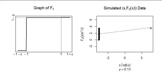
Let $\epsilon$ be a (tiny) positive number and consider now any continuous variable $X$ with support on $[-1-\epsilon,-1]\cup[1,1+\epsilon].$ Suppose $\Pr(X \le 0) = 1-p$ and (therefore) $\Pr(X \gt 0) = p.$ Let's compute the correlation by finding the relevant moments.

In the right hand plot, both variables have been standardized to unit variance: their correlation coefficient is the slope of the least squares line shown. Here, $p=1/2.$

Clearly $F_X(x)=0$ for $x \lt -1-\epsilon,$ rises continuously to a value of $1-p$ at $x=-1,$ is level at that value for $-1\lt x \lt 1,$ and then rises continuously to $1$ by the time $x$ reaches $1+\epsilon.$ Again, since $X$ is a continuous random variable, $F_X(X)$ is a uniform random variable on $[0,1].$ Also, since $X$ is closely approximated by a binary random variable $Y$ with $\Pr(Y=1)=p$ and $\Pr(Y=-1)=-p,$ their variances will be close and $\operatorname{Var}(Y)=4p(1-p).$

The covariance is a little trickier. Compute

$$\operatorname{Cov}(X, F_X(X)) = E[X(F_X-1/2)] = \int_{-1-\epsilon}^{-1} x (F_X(x)-1/2)f_X(x)\,\mathrm{d}x + \int_1^{1+\epsilon} x (F_X(x)-1/2)f_X(x)\,\mathrm{d}x.$$

Integrate these by parts by splitting the integrands into $x$ and all the rest. The result is $p(1-p) + O(\epsilon).$ Consequently

$$\operatorname{Cor}(X, F_X(X)) = \frac{p(1-p)/2 + O(\epsilon)} {\sqrt{4p(1-p)+O(\epsilon)}\sqrt{1/12}} = \sqrt{3p(1-p)/4} + O(\epsilon).$$

This can be made as close to $0$ as we might like by making $p$ close to either $0$ or $1$ and shrinking $\epsilon.$ Consequently, any lower bound on the correlation cannot be positive.

Most of the density of $X$ has been pushed up against $\pm 1$ by shrinking $\epsilon.$ Now $p=1/200.$ The correlation has reduced from $0.87$ in the first figure to $0.13$ here.

Finally, since $F_X$ is a non-decreasing function, the correlation of $X$ with $F_X$ cannot be negative. Coupled with the preceding observation we conclude

Universal bounds for the correlation of $(X, F_X(X))$ are $0$ and $1.$ These are the best possible.

In fact, $0$ cannot be attained. (The intuitively obvious case would be to take the limits as $p\to 0$ and $\epsilon\to 0^+$ in the second example, but this reduces $X$ to a constant, where the correlation is undefined.)