A common way to define which estimator is better is to compare them on their mean squared error (MSE). Loosely speaking, MSE measures the average amount by which an estimate differs from the true value. More technically, MSE is defined as follows, for a $\hat\theta$ that estimates a true value $\theta$. (That $\theta$ has nothing to do with angles and is just the preferred Greek letter in statistics.)
$$
MSE(\hat\theta) = \mathbb{E}\bigg[
\big(\theta - \hat\theta\big)^2
\bigg]
$$
MSE has a convenient decomposition into the bias of the estimator and the variance of the estimator (the so-called "bias-variance decomposition" or "bias-variance" tradeoff that you might hear in machine learning circles).
$$
MSE(\hat\theta) = bias(\hat\theta)^2 + var(\hat\theta) = \big(\mathbb{E}\big[\theta - \hat\theta\big]\big)^2 + var(\hat\theta)
$$
When we know that an estimator has desirable MSE in a situation like the one we face, we might choose that estimator, so let's compare your proposed estimator with the usual $\bar X$ sample mean in a situation like you've described. I've worked this out for $X\sim\chi^2_5$.
We know the bias and variance of $\bar X$. With a small caveat that these quantities have to be defined (which is a reasonable assumption in many situations):
$$
bias(\bar X) = 0\\
var(\bar X) = \dfrac{var(X)}{n}
$$
In this setting, $var(X) = 10$, so $MSE(\bar X) = bias(\bar X)^2 + var(\bar X) = 0^2 + \dfrac{10}{n} = \dfrac{10}{n}$.
To estimate the MSE for your proposed estimator that applies a Box-Cox transformation, calculates the mean of the transformed data, and does the inverse of the Box-Cox transformation, I turned to a simulation in R software. I started by simulating many observations from $\chi^2_5$ and determining that the right Box-Cox transformation to achieve normality was about a cube-root.
library(MASS)
set.seed(2022)
N <- 30000
x <- rchisq(N, 5)
bc <- MASS::boxcox(x ~ 1)
bc$x[which(bc$y == max(bc$y))] # This tells me that the right Box-Cox
                               # transformation is about a cube root.
                               # 0.3-ish is close enough to 1/3
Next, I simulated $1000$ small samples from $\chi^2_5$, calculated your estimate of variance (cube root the data, calculate the mean of the transformed data, cube the mean of the transformed data) each time, and calculated the mean squared error of those $1000$ estimates, knowing that the true mean is $5$.
# Now let's simulate the MSE of your proposed estimator
#
B <- 1000 # Iterations
N <- 3 # Sample size...fiddle with this and check out what happens :)
means_bc <- rep(NA, B)
for (i in 1:B){

  # Simulate some data
  #
  x <- rchisq(N, 5)

  # Apply the cube-root transform
  #
  x_prime <- x^(1/3)

  # Calculate the mean of x_prime
  #
  m <- mean(x_prime)

  # Now cube the mean and save that value as an estimate of the mean of X
  #
  means_bc[i] <- m^3

  print(i)
}

# Calculate the MSE of "means" (using the Box-Cox transform)
#
mse_bc <- (mean(means_bc - 5))^2 + var(means_bc)

# Calculate the MSE of the usual x-bar estimator
# X-bar is unbiased
# Analytic solution for var(X-bar) is sigma/N
#
mse_usual <- 0^2 + 2*5/N

hist(means_bc)
abline(v = mse_usual, col = 'blue')
abline(v = mse_bc, col = 'black')
The histogram gives the distribution of values calculated your way, the black line is the MSE of your approach, and the blue line is the MSE of $\bar X$.
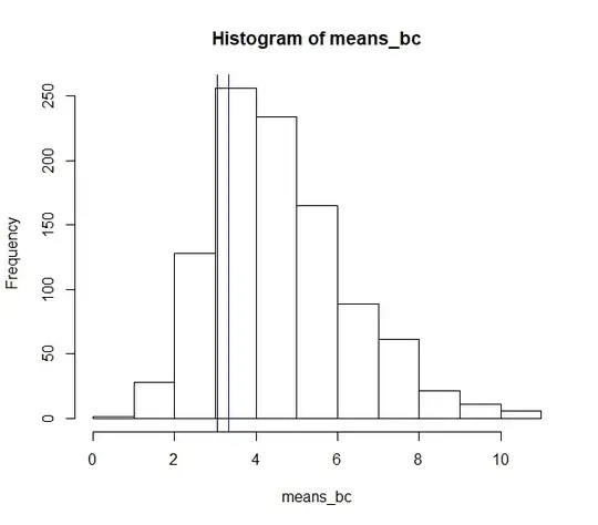
Your estimator gives a lower MSE than the usual $\bar X$ estimator. I was surprised.
This doesn't mean that we should go Box-Cox transform our data, calculate the mean, and then invert the Box-Cox transformation. I used a contrived example with $\chi^2_5$ data, and $\chi^2$ distributions usually arise in hypothesis testing, not real data generation. Further, the Box-Cox transformation is pretty effective in this case, yet it need not be in other cases.
However, this result so surprised me that I had to share.

