2

I have a set of incomplete data for wealth of a given population. Whilst I have the wealth of these individuals (around 27% of the population), I do not have the wealth of every individual. I do have the total wealth in circulation (that is, the total amount of money present within the system) but not how this is distributed. I also know the population size.

I would like to find a given individual's percentile wealth, as it relates to the population. Would this simply be calculated upon the sample and then stated as likely according to a confidence interval with x% margin of error?

The problem I have is as follows. My suspicion is that the wealth is not normally distributed but I cannot prove this. As such, would I simply assume normality and caveat the conclusion therein or is there a tool by which I could better assess the distribution and then calculate the likely percentile from there?

To summarise, data I have:

  • Wealth of individuals in a random sample (27% of the population)
  • The population size
  • The total wealth in the population

Data I do not have:

  • How the wealth is distributed in the population

What I would like to find:

  • The percentile wealth of the sample

Thank you.

whuber
  • 281,159
  • 54
  • 637
  • 1,101
twelfth
  • 25
  • 4
  • 1
    Is your sample random or not? If it's random, you can apply standard statistical techniques for making inferences about the population. Which ones to apply depend on what assumptions you can make about the population distribution (ranging from no assumptions to a specific distributional shape). If the sample is not random, you will need to describe in detail how it might be related to the population in order to obtain any kind of an accurate answer. BTW, unless this population is highly unusual, a Normal distribution would be a poor model. – whuber Feb 04 '22 at 15:45
  • Hi @whuber. My sample is random. I am not sure what assumption I can make of the population distribution as the only information I have of it is its size and the total wealth in the population. Could you explain why normal distribution would be a poor model in this case please? Thank you for your comment. – twelfth Feb 04 '22 at 15:50
  • 3
    Income distributions are usually highly skewed, which is true of no Normal distribution. How large is your sample, exactly? Unless it is truly tiny, what is the problem with using its percentiles to estimate the population percentiles? – whuber Feb 04 '22 at 15:59
  • Hi @whuber. Thank you for the explanation, that makes it clearer for me. My sample size is 6,750. The population size is 25,000. I suppose my only issue was that I thought percentile calculations assumed a normal distribution, but I suppose this is incorrect? In that case, I could therefore simply estimate percentiles with a given (1.02% I believe) margin of error at the 95% confidence interval, if I understand correctly? – twelfth Feb 04 '22 at 16:02
  • 1
    Percentile calculations--properly conducted!--depend on *no* distributional assumptions at all. You estimate a percentile in terms of proportions found in the sample. As far as standard errors go, your sample is such a large fraction of the population that you can benefit from applying "finite population corrections" to the usual standard error formulas. Depending on what you really need to accomplish, something as simple as plotting the empirical CDF with KS-like error bounds might do the job nicely. – whuber Feb 04 '22 at 16:05
  • Thank you very much for your responses, that alleviates a lot of stress for me! I have taken a look at finite population corrections and thank you for pointing that out, I would have missed this otherwise. I have a question regarding the final sentence; I have looked into ECDF now (here: https://towardsdatascience.com/what-why-and-how-to-read-empirical-cdf-123e2b922480) but could not find resources regarding the KS-like error bounds you mention. If you could point me in that direction, I would very much appreciate it! – twelfth Feb 04 '22 at 16:12
  • 1
    That last remark was somewhat speculative. The KS test is based on knowing the largest amount by which the ECDF of a sample will differ from the underlying CDF at any point. Presumably one could develop a finite population correction to narrow that KS critical value for samples without replacement. I think that would have to be worked out through simulation: the analytical approach looks formidable. But maybe the unadjusted bounds would be acceptable in your application. Look up the theory of the Kolmogorov-Smirnov test to learn more. – whuber Feb 04 '22 at 16:14
  • Thank you very much for that! I will do so. That about answers my question too, I very much appreciate your response. My apologies, I am unable to upvote comments yet but thank you all the same! – twelfth Feb 04 '22 at 16:16

1 Answers1

3

The question concerns a non-parametric estimation of a finite population distribution based on a random sample (without replacement) comprising an appreciable fraction of that population.

The empirical cumulative distribution function (ECDF) is a fine non-parametric estimator. It estimates the proportion of the population at or below any number $x$ to be the proportion in the sample at or below $x.$

Ordinarily, for a sample with replacement, one would use the Kolmogorov Distribution to construct confidence bands around the ECDF. These bands are obtained by raising and lowering the graph of the ECDF by an amount $D,$ the critical value of a KS test. For $100(1-\alpha)\%$ confidence, $D$ is the $1-\alpha$ quantile of the Kolmogorov distribution, divided by $\sqrt{n}.$ (The bands obviously can be cut off by $1$ at the top and $0$ at the bottom, as shown in the figures below.)

A standard correction factor for estimating standard errors of the mean in large samples of size $n$ without replacement from populations of size $N$ is to multiply them by $\sqrt{(N-n)/(N-1).}$ See our explanation at Explanation of finite population correction factor?.

As an ad hoc attempt at a solution, I have adjusted the critical value of $D$ in the same way. Simulations indicate this adjustment works provided $N$ is large -- typically over a thousand or so. "Works" means that the bands are at the proper distances to achieve the intended confidence level.

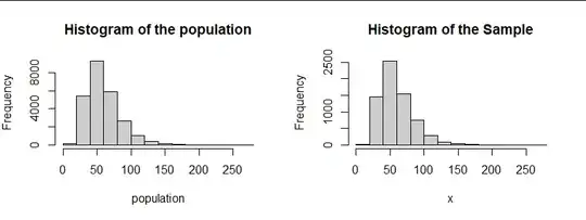
The first figure shows a skewed population characteristic of incomes. It has $25,000$ values. At the right of that figure is a histogram of a random sample of size $6,750$ (without replacement) from that population. (Comments to the question indicate these are the quantities the OP actually has.) Because it's a large sample, its histogram has almost the same shape as the population histogram.

Figure 1

The next figure shows the ECDF (at left) for the sample with the 95% confidence bands (as adjusted for the finite population). It's hard to distinguish the ECDF itself (in black) from the bands, so at the right I have plotted the difference between the sample ECDF and the population ECDF. When the red and blue lines at the right are set at the correct heights, then in 95% of such random samples, the entire black graph of deviations will lie between those bands. Thus, although in practice we never know the population distribution, when we look at the left plot (which is based only on information about the sample), we get a good sense of how reliably that sample represents any quantile of the population.

Figure 2

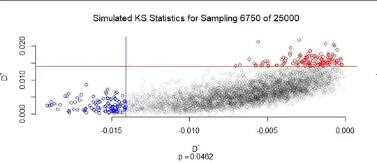
For the final figure I have created five thousand random samples of the same population (a quantity I could generate and analyze in a couple of seconds). For each one I recorded the largest positive deviation relative to the population distribution, $D^+,$ and the greatest negative deviation, $D^-.$ (The KS statistic is the larger of $D^+$ and $-D^-.$) Thus, each sample contributes on point $(D^-, D^+)$ to this plot. Samples where one (or potentially both) deviations fell beyond the confidence bands are shown in red and blue. As noted at the bottom, this is $0.0462 = 4.62\%$ of all the samples. Because this number is so close to $5\%,$ we may conclude that the method of computing the critical value of $D$ is accurate.

Figure 3

The method I used is shown in the code below. It calculates the critical value of $D$ by (a) implementing the CDF of the Kolmogorov distribution, (b) inverting it with a root finder, and (c) applying a correction recommended in the Wikipedia article. The correction makes little difference for a sample of this size, but helps a little bit for smaller samples. Once the sample size drops down to the hundreds, though, these calculations are too conservative in the sense that their critical value is too large; equivalently, the actual confidence of this test is higher than its nominal level.

You can change obvious parts of this code to study any sampling situation you might face. Two things to bear in mind are (1) obtaining tied values in the sample should be a rare event and (2) other than that, it doesn't matter what you assume for the population distribution.

#
# The Kolmogorov CDF.
#
pK <- Vectorize(function(x) {
  x <- pmin(4, pmax(2^(-4), x))
  kmax <- ceiling(3 * x)
  k <- seq(1, 2*kmax-1, by=2)
  sum(exp(-(k * pi / x)^2 / 8)) * sqrt(2*pi) / x
})
#
# The percentage point function (inverse CDF)
#
qK <- Vectorize(function(q, ...) {
  q <- pmax(1e-13, pmin(1 - 1e-13, q))
  f <- function(x) pK(x) - q
  uniroot(f, c(2^(-4), 4), ...)$root
})
#
# An adjustment to make `pK` more accurate for smaller `n`.
#
adjust <- function(x, n) (x - 1/sqrt(36*n)) / (1 + 0.25/n)
#
# An example.
#
N <- 25e3
n <- 6.75e3
alpha <- 0.05
population <- exp(rnorm(N, 4, 0.4))
#
# Compute some objects for the plots.
#
F.0 <- ecdf(population)
D <- adjust(qK(1-alpha), n) / sqrt(n) * sqrt((N-n)/(N-1))
#
# Sample from the population.
#
set.seed(17)
x <- sample(population, n)
F.x <- ecdf(x)

par(mfrow=c(1,2))
#
# Figure 1: histograms.
#
hist(population, col=gray(.8), main="Histogram of the population")
hist(x, col=gray(.8), main="Histogram of the Sample")
#
# Figure 2: how the confidence bands work.
#
plot(range(x), 0:1, type="n", bty="n", yaxp=c(0, 1, 2), 
     main="Sample Distribution", xlab="Income", ylab="Proportion Below")

x.0 <- seq(min(x), max(x), length.out=201)
y <- F.x(x.0)

polygon(c(x.0, rev(x.0)), c(pmin(1, y+D), pmax(0, rev(y)-D)), col=gray(.80), border=NA)
# curve(F.x(x), add=TRUE, lwd=2, n=201)
curve(F.x(x), add=TRUE, n=501)
curve(pmin(1, F.x(x) + D), add=TRUE, col="Red", n=501)
curve(pmax(0, F.x(x) - D), add=TRUE, col="Blue", n=501)


plot(range(x), 2*D*c(-1,1), type="n", bty="n", xlab="Value", ylab="Deviation",
     main=bquote(paste(.(100*(1-alpha)), "% Confidence Interval")))
abline(h = D*c(-1,1), col = c("Blue", "Red"))
curve(F.x(x) - F.0(x), min(x), max(x), add=TRUE, n=501)
par(mfrow=c(1,1))
#------------------------------------------------------------------------------#
#
# A simulation.
#
N <- 25e3     # Population size
n <- 6.75e3   # Sample size
alpha <- 0.05 # Test size: confidence is 100*(1-alpha).

set.seed(17)
population <- exp(rnorm(N, 4, 0.4))
F.0 <- ecdf(population)
#
# Draw samples repeatedly and compare their ECDFs to the population CDF.
#
sim <- replicate(5e3, {
  x <- sort(sample(population, n))
  y <- (1:n) / (n+1) - F.0(x)
  range(y)
})
#
# Assess and plot the results.
#
D <- adjust(qK(1-alpha), n) / sqrt(n) * sqrt((N-n)/N)
p <- mean((ilow <- sim[1,] < -D) | (ihigh <- sim[2, ] > D))
plot(t(sim), bty="n", col=ifelse(ilow, "Blue", ifelse(ihigh, "Red", "#00000020")),
     main=bquote(paste("Simulated KS Statistics for Sampling ", .(n), " of ", .(N))),
     sub=bquote(p==.(signif(p, 3))),
     xlab=expression(D^paste("-")), ylab=expression(D^paste("+")))

abline(h = D*c(-1,1), v = D*c(-1,1), col=c("Blue", "Red"))
whuber
  • 281,159
  • 54
  • 637
  • 1,101
  • Thank you very much. What a clear, concise, and thorough answer. This helps immeasurably and I cannot thank you enough. I just wished to clarify; as well as the above sample of 6,750, I have a secondary sample obtained at an earlier date (thus with a different income distribution) but of the same population size. This secondary sample size is 150. Would I be correct in thinking the ECDF would not be applicable in this case (and thus should simply proceed in calculating the percentile ranks) or is this a different problem entirely which I should pose as a separate question? Thank you again! – twelfth Feb 05 '22 at 12:06
  • 1
    The ECDF is *always* applicable. With a sample of $150,$ though, you will find the critical value of $D$ is fairly large, leading to wide confidence bands. A finite population adjustment is no longer needed, because $150$ is such a small fraction of $25,000.$ The nominal 95% bands actually achieve 96% coverage (that is, the computed $D$ is a little too small, but not by much). The critical value is almost $11\%.$ If you were to focus on just a few important quantiles, though, you can get substantially narrower confidence intervals. – whuber Feb 05 '22 at 14:10
  • Thank you. I was under the mistaken impression that the ECDF was only applicable to large samples (proportionate to the population size) but was mixing this up with the finite population adjustment. In that case, I shall probably narrow the focus as you state by looking at just a few quantiles. – twelfth Feb 05 '22 at 14:17
  • 1
    The literature on nonparametric statistical methods explains how to construct intervals for quantile estimates. At https://stats.stackexchange.com/a/160148/919 I present the standard analysis for a single quantile. For simultaneous intervals around multiple quantiles, the concern is that the sample estimates will be correlated. But if the quantiles are widely spaced and the sample size isn't terribly small, perhaps that correlation can be neglected. – whuber Feb 05 '22 at 14:21
  • Thank you for reference to your answer. I will utilise this to aid construction of the intervals for this smaller sample. I am not sure how widely spaced the quantiles are but shall bear what you say in mind with respect to this. – twelfth Feb 05 '22 at 14:43