8

$\newcommand{\icol}[1]{% inline column vector \left(\begin{smallmatrix}#1\end{smallmatrix}\right)% }$

Scenario:

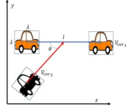
Let's consider a road segment on which there is continuous flow of cars circulating at a constant speed $V_{car_1}$ and where cars are all equally spaced by a distance $l$. Now imagine that a car 2 is crossing the road at a constant speed $V_{car_2}$ with an intersection angle $\theta$. Assuming both cars having a square shape of length $\lambda$, the goal is to estimate the probability of collision.

enter image description here

Method 1:

The probability of collision is given by: $$ P_{collision} = P_{car2\_hits\_car1} \lor P_{car1\_hits\_car2} $$

$$ \\P_{car2\_hits\_car1} \approx \frac{2\lambda}{l} \\P_{car1\_hits\_car2} \approx crossing\_time \,\frac{|V_{car_1}-V_{car_2}\,cos(\theta)|}{l} = \frac{2\lambda \,|V_{car_1}-V_{car_2}\,cos(\theta)|}{l\, V_{car_2}\,sin (\theta)} $$ which leads to: $$P_{col\_method\_1} \approx \frac{2 \lambda}{l}\left(1+ \frac{|V_{car_1}-V_{car_2}cos(\theta)|}{V_{car_2}sin (\theta)}\right)$$

Method 2:

Now for some reasons, we want to estimate this probability of collision using a different method. The car 1 position probability density is estimated using a kernel density estimation. The function $f(x,y)$ gives the probability of the center of the car 1 being at coordinates $(x , y)$.

$f$ is obtained using traffic observation data: each car 1 trajectory observation on the segment of length $l$ is represented by a uniformly time sampled (dt = 0.01 seconds) series of position $(x_1(t), y_1(t))$. Multiple trajectory observation (taking a year of observations for example) are concatenated and $f$ is obtained by fitting a kernel density estimate on these concatenated observations (using scikit-learn kde in practice). We then have: $$ \int\limits_{min(y_1)}^{max(y_1)} \int\limits_{0}^{l}{f\left(x, y\right) \,dx\,dy} = 1 $$

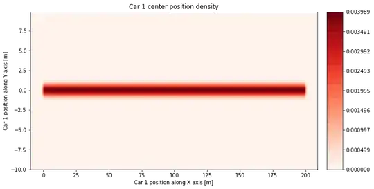
Here is an example of contour plot for an estimated density f: enter image description here

Now, let's consider $C_2 = \icol{x_2\\y_2}$ the coordinates of the car 2, we have: $$ C_2(t) = \begin{pmatrix} x_2(t)\\ y_2(t) \end{pmatrix} = \begin{pmatrix} x_{2_0}+V_2 cos(\theta) t\\ y_{2_0}+V_2 sin(\theta) t \end{pmatrix} $$

Considering that the car 1 always comes from the left of the crossing point and that the car2 always come from the bottom, I expect the probability of collision to be: $$ P_{collision} = P_{car2\_hits\_car1} \lor P_{car1\_hits\_car2} $$ Using density integration: $$ \\P_{car2\_hits\_car1} \approx \int\limits_{0}^{+\infty} \int\limits_{y_2(t)-\lambda}^{y_2(t)+\lambda}{f\left(x_2(t)-\lambda, y\right) \,dy\,dt} \\P_{car1\_hits\_car2} \approx \int\limits_{0}^{+\infty} \int\limits_{x_2(t)-\lambda}^{x_2(t)+\lambda}{f\left(x, y_2(t)+\lambda\right) \,dx\,dt} $$ $$ P_{col\_method\_2} \approx \int\limits_{0}^{+\infty} \int\limits_{y_2(t)-\lambda}^{y_2(t)+\lambda}{f\left(x_2(t)-\lambda, y\right) \,dy\,dt} + \int\limits_{0}^{+\infty} \int\limits_{x_2(t)-\lambda}^{x_2(t)+\lambda}{f\left(x, y_2(t)+\lambda\right) \,dx\,dt} $$

Motivation for the choice of integral bounds:

integration bounds motivation Basically at rach dt, we integrate the probability of a car1 beeing on the blue line and on the red line.

Results:

The obtained results between the 2 methods are different and the following relation has been found empirically: $$ P_{col\_method\_1} = \frac{V_{car_2} sin \theta +|V_{car_1} - V_{car_2}cos\theta|}{2}P_{col\_method\_2} $$

For example considering both cars of size $\lambda=3$ running at $V_1=V_2=10m/s$ crossing at a $\theta = 90deg$ and taking $l=100m$ gives: $$ \\ P_{col\_method\_1} = 0.12 \\ P_{col\_method\_2} = 0.012 $$

Question:

While I understand that there need to be a "scaling factor" that needs to be in m/s to obtain correct units for the second method, I can't explain its formula. Does anyone have an explanation for it?

The code is available as a python notebook: https://colab.research.google.com/drive/1ypeq7SSPUGqMyxn1Dxs6_lhenCnCTUFD?usp=sharing

Info:

A quick Monte-Carlo simulation shows that the method 1 is giving the right probabilities.

Benoit Fgt
  • 113
  • 7
  • Why does the probability that car2 hits car1 not dependent on theta? It seems the smaller theta is, the greater the chance of collision? – barrycarter Feb 04 '22 at 12:56
  • That's a good point you are raising. The reason is that we consider the shape of the car 2 to always be aligned with the road (like if the theta is equal to 0deg or 90deg). This introduces a small error in the computation (it's small enough for our application) but it simplifies the maths quite a lot. – Benoit Fgt Feb 04 '22 at 13:02
  • I don't think that's true. If theta is small, there's much more time for car2 to hit car1. If theta is 90 degrees, the chance is minimal, but as theta approaches 0 you can virtually guarantee car2 will hit car1 (assuming car2's speed is independent of theta) – barrycarter Feb 04 '22 at 13:06
  • In my opinion, no matter the intersection angle, when we assume both square to be aligned with the road, the probability of having car 2 hitting car 1 is $2\lambda/l$. Something I should add to the post is that I have monte carlo verified the results and the method 1 gives a good probability of collision. – Benoit Fgt Feb 04 '22 at 13:35
  • 2
    I cannot make sense of Method 2, because it seems not to incorporate relevant information about car lengths or speeds. In particular, what aspects of traffic flow specifically does a "probability density" describe?? How would a given "density" function distinguish a parade of cars of length $L$ moving at speed $s$ from cars of length $L/100$ moving at speed $100s,$ for instance? Intuitively, the chance of a collision is certain in the latter case. – whuber Feb 04 '22 at 14:21
  • You are right speed and intersection angle information are missing in the probability density estimation. Concerning the size of the car, I think that it is included into the integral bounds. – Benoit Fgt Feb 04 '22 at 14:36
  • 1
    It still isn't clear what this "probability density" might be. Exactly how do you define it in terms of the dynamics of the traffic? I suspect you might be trying to describe something else, such as the intensity of a stochastic process, using the term "probability density." – whuber Feb 04 '22 at 15:49
  • I have added some context on the estimation of f (let me know if it's not clear), it seems to me that the term probability density is correct. – Benoit Fgt Feb 04 '22 at 22:20
  • It cannot be a probability distribution. Suppose exactly one car passes along this segment in the entire year: the result of your KDE of the samples of that car's coordinates will still look like your graphic, even though the chance of a collision is essentially zero. – whuber Feb 04 '22 at 23:06
  • If there is only one observation a year, it means that the speed of the car is $\frac{l}{3600 \cdot 24 \cdot 365}$ so the car1 will still be somewhere on the segment when the car 2 will cross and the probability to be hit by car 2 is still $\frac{2\lambda}{l}$. But I agree that the KDE result will be exactly the same if there are multiple observations. (In practice we want to apply it in 3D for airplanes so you have a bigger dispersion in all dimensions but first I need to understand a simple 2D case.) – Benoit Fgt Feb 05 '22 at 08:14
  • Benoit, could you give a bit more background about the problem that is underlying this question? There are quite some loose ends and it is difficult to know where to start in answering this question (specific solving the puzzle or abstract explaining the principles of computing collision rates). Is this a little case study to practice the mathematical principles or is this some starting point for a concrete application? – Sextus Empiricus Feb 11 '22 at 15:57
  • @SextusEmpiricus, it is the starting point for a concrete application. Basically, we want to compute the probability of having mid-air collisions: we have a scenario where there is an air route segment (the segment is curved, aircraft are having different speeds, and not exactly flying the route) flown by aircraft and from time to time, we might have an intruder crossing this route. Now the goal is to "simulate" an intruder trajectory and compute the probability of collision (this part is easier as we assume the intruder to have straight trajectory with constant speeds / rate of climb). – Benoit Fgt Feb 11 '22 at 18:51
  • @SextusEmpiricus so the first thing we did was to obtain the density function of the aircraft on the route for a defined volume (similarly than what I did for car 1). – Benoit Fgt Feb 11 '22 at 18:58
  • @SextusEmpiricus I confirm that the result of this integral is 1 in my application. – Benoit Fgt Feb 16 '22 at 15:41
  • @BenoitFgt I think that the factor 20 difference is because you need to incorporate the velocity (to convert time in distance) and use the appropriate time frame or effective velocity. Currently in the final answer I have an integral that computes in the same way as method 1. The section 'method variant 2' is also helpful. – Sextus Empiricus Feb 16 '22 at 15:54
  • I will implement your latest update latter today and let you know what I get. – Benoit Fgt Feb 16 '22 at 15:56
  • @SextusEmpiricus, I have implemented the path integral you mentioned but somehow my result is still different. I have detailed my integration, can you see any wrong step? – Benoit Fgt Feb 16 '22 at 21:44
  • There's a factor $v \sin \theta$ missing. The integral over $ds$ should result in the length of the path which is the total speed of car 2 divided by the y component of that speed multiplied by the width of the stream. – Sextus Empiricus Feb 16 '22 at 21:54
  • @SextusEmpiricus apologize my late answer but I am still banging my head around and trying to make sense of everything. In your method 1 you obtain $p_{col} = \frac{2*\lambda}{l\cos\theta'}$ but if compare with my formulation of the method 1, I obtain $p_{col} = \frac{2 \lambda}{l}(1+ \cot\theta')$. – Benoit Fgt Feb 17 '22 at 21:02
  • See the second image where I wrote 'distance between stream 1 blocks'. Let's call this $l^\prime$. You can view $l$ and $l^\prime$ as part of a right angled triangle (where $l$ is the diagonal and $l^\prime$ one of the right sides) with the same ratio as the triangle made by the velocities of the block 2 in the co-moving frame (the triangle made out of the total velocity vector and the X and y components)... – Sextus Empiricus Feb 17 '22 at 22:27
  • ... So you get $$\frac{\text{diagonal}}{\text{right side}} = \frac{l}{l^\prime} = \frac{|v_2^\prime|}{v_{2,y}^\prime} = \frac{\sqrt{(v_2 \text{sin}\, \theta)^2+(v_2 \text{cos}\,\theta -v_1)^2}}{v_2 \text{sin}\, \theta}$$ Here I use $v^\prime$ to denote the velocity in the co-moving frame of reference (I did not do this in the answer and the velocities might sometimes be confusing, maybe in some later edit of even more will follow). – Sextus Empiricus Feb 17 '22 at 22:30
  • you need to spell out what's known about car 1 in the method 2 if you want people help you. nobody's going to parse your code for this. from your brief description in the question it appears that you know its speed and the distance between cars on the road, then the only thing left out would be the relative location to car 2, but it's not obvious. it's not clear whether there is a noise in locations. without noise a single observation of a car 1 would tell you exactly whether you are colliding or not. as it is the problem is not stated clearly – Aksakal Feb 21 '22 at 17:11

2 Answers2

6

Related scattering theory and free path length

Change frame of reference

You can compute your method 1 more easily by switching the frame of reference to a co-moving frame along with the stream of cars.
illustration of co moving frame

If the car 1 has the velocity $\vec{v}_1$ and car 2 have the velocity $\vec{v}_2$ then in the co-moving frame the relative speed between the cars is $\vec{u} = \vec{v}_1 - \vec{v}_2$ with the components

$$\begin{array}{} u_{x,2} &=& v_2 \text{cos}\,\theta -v_1 \\ u_{y,2} &=& v_2 \text{sin}\, \theta \\ \end{array}$$

Then we consider a different angle $\theta^\prime$ at which the car2 is passing the stream while the cars 2 are standing still. This angle is related to the new vertical and horizontal velocities in the co-moving frame of reference.

frame of reference

In 'Motivation for the choice of integral bounds' you work with two components:

  1. The probability of the car 1 hitting car 2, which relates to $u_{x}$ the relative horizontal speed at which car 1 approaches car 2.

  2. The probability of the car 2 hitting car 1, which relates to the $u_{y}$ the relative vertical speed at which car 1 crosses the stream.

In the viewpoint of the frame of reference that is co-moving with the cars 1, you can see that this idea of two components 'car 1 hitting car 2' and 'car 2 hitting car 1' is confusing. One should not add the horizontal and vertical components $u_{x}$ and $u_{y}$ together (which is like computing the Manhattan distance), but you should use the Euclidian measure for the distance traveled by car 2 relative to the cars in the stream $\sqrt{u_{x}^2 + u_{y}^2}$.

Effective cross-section

To compute the collision rate or collision probability, you will have to consider the effective cross-section of the car moving through the stream.

If you would do this accurately you will have to determine the distances $d_1$ and $d_2$ which are the distances between the point where the two cars are just touching and lines through the centers of the two cars, these lines are drawn in the direction of travel.

To compute these distances is a bit annoying and you have to consider both the angles $\theta$ and $\theta^\prime$. And, there are different cases, for instance, car 2 might hit the other car on the left or the right side depending on the angle.

You could approximate the distance with $\lambda$ if you simplify the shape of the cars as spheres with diameter $\lambda$. The cross section will then be twice this distance because the car 2 can hit the car 1 on the left and on the right.

The distance between the cars 1 or the density in the stream.

If we approach the stream at an angle than the distance between the cars in the stream becomes smaller. In the figure below you see that this distance is not $l$ but instead $l \sin \, \theta^\prime$.

cross section

Probability of hit with method 1

The probability that a car 2 hits another car in the stream is then

$$\frac{\text{cross-section}}{\text{path-width}} \approx \frac{2 \lambda}{l \cdot \sin \, \theta^\prime}$$

and with $$\sin \theta^\prime = \frac{u_{y}}{\sqrt{{u_{x}}^2+{u_{y}}^2}}$$

we can rewrite it as

$$\frac{\text{cross-section}}{\text{path-width}} \approx \frac{2 \lambda}{l} \sqrt{ 1 + \left( \frac{v_2 \cos \, \theta - v_1}{v_2 \sin \, \theta} \right)^2}$$

It is possible that this ratio becomes larger than 1 when the cross-section becomes larger than the path width. In that case a collision is certain (if the cars in the stream are with constant distance/gaps in between).

Method 2, using density

With the method you will have to compute the area that is swept by car 2 and integrate over that area the density of the cars 1 (which is more easy if this density is constant).

using density 2

Note that the angle of the path changes the area of the path. The integral that you compute, and the motivation for it, is not so clear. It is like you are computing the area of the path of a 1 dimensional line. That area is not dependent on the angle of the car 1. But, it is wrong to use a line. You need to consider the entire block.

See in the image below how car 2, if it would be taking an alternative path, would sweep a different area of the stream. Also the velocity of cars 1 plays a role because they change the effective angle $\theta^\prime$ which will change the size of the area that the car 2 sweeps through the stream.
 using density 1

Note: in the image $\cos \theta^\prime$ should be $\sin \theta^\prime$. This will be edited later.

The image above depicts a stream of uniform density, but you can also consider a nonuniform density in which case you perform an integration over infinitely small slabs.

So this area is equal to

$$w \cdot x = w \cdot \frac{2\lambda}{\sin\, \theta^\prime}$$

You will have to multiply by the density of the cars which is 1 car per block of size $w$ by $l$, ie $\rho = 1/(l\cdot w)$ and you will end up with the same expression as method 1.

$$w \cdot x \cdot \rho = w \cdot \frac{2\lambda}{\sin\, \theta^\prime} \cdot \frac{1}{l\cdot w} = \frac{2\lambda}{l \cdot \sin\, \theta^\prime} $$

Method 2 variant

We can also compute the integral from method 2 in the stationary frame of reference.

The area computed above is using the area of the parallelogram as (height times width). This can be done in two ways:

  • one is $w \cdot x$ where $w$ is the width of the stream and $x$ the length of the intersection.
  • Another way would be to multiply the cross-section $2\lambda$ with the length of the path which is depending of the width of the stream and the angle $\theta^\prime$.

This length of the path can be seen as an effective velocity relating how many area the car 2 effectively travels in the co-moving frame of reference of the car 1 stream.

Instead of computing the area in the frame of reference of the co-moving frame we could also compute the area in the stationary frame of reference.

  • In the stationary frame of reference the distance traveled is $$\Delta x \cdot \text{cross-section} = v_2 \Delta t \cdot \text{cross-section}$$

  • In the co-moving frame of reference the distance traveled is $$v_{effective} \Delta t \cdot \text{cross-section}$$

So we could compute the effective area as the area in the stationary frame of reference multiplied by a factor

$$v_2 \Delta t \cdot \text{cross-section} \cdot \frac{v_{effective}}{v_2}$$

This factor at the end is the ratio of the difference in speeds of car 1 and car 2 in the numerator and the speed of car 1 in the denominator

$$ \frac{v_{effective}}{v_2} = \frac{\sqrt{(v_2 \cos \, \theta -v_1)^2+(v_2 \sin \, \theta)^2}}{v_2}$$

The time traveled in the stream of width $w$ is relating to another factor

$$\Delta t = \frac{w}{v_2 \sin \, \theta}$$

If you put those together you get the same result again.


If you like to compute an integral to account for some nonhomogeneous density then you could use a path integral

$$ \int \text{cross-section}(s) \rho(s) \frac{|\vec{v}_1(s)-\vec{v}_2(s)|}{|\vec{v}_2(s)|} \text{d}\, s$$

Where the velocities are now considered as vectors $\vec{v}_1$ and $\vec{v}_2$, and the vertical bars $|\cdot|$ denotes the magnitude.

If the cross-section $2 \lambda$, density $\rho = \frac{1}{l\cdot w}$ and speeds are constant then we can take them outside of te integral and we end with

$$ \begin{array}{} \text{cross-section} \cdot \rho \cdot \frac{|\vec{v}_1-\vec{v}_2|}{|\vec{v}_2|} \cdot \int \text{d}\, s &=& \overbrace{\left(2 \lambda\right)}^{\text{cross-section}} \cdot \overbrace{\left( \frac{1}{l \cdot w} \right)}^{\text{density}} \cdot \overbrace{\left(\frac{|\vec{v}_1-\vec{v}_2|}{|\vec{v}_2|}\right)}^{\text{velocity factor}} \cdot \overbrace{\left( w \frac{|\vec{v}_2|}{{v}_{2,y}} \right)}^{\text{path length $\int \text{d}s$}} \\ &=& \frac{2 \lambda}{l} \frac{|\vec{v}_1-\vec{v}_2|}{{v}_{2,y}} \\ &=& \frac{2 \lambda}{l} \frac{\sqrt{(v_2 \sin \theta)^2 + (v_2 \cos \theta- v_1)^2}}{v_2 \sin \theta} \end{array}$$
integration

Note that this gives the average number of collisions. The meaning of an average is different depending on the distribution of the cars in the stream. (See: What distribution to use to model time before a train arrives?)

In your final application with airplanes you might consider the collisions between two streams. Then you can have an integral over the space and use the concentrations of both streams

$$ \iint \rho_1(x,y) \rho_2(x,y) \text{cross-section}(x,y) {|\vec{v}_1(x,y)-\vec{v}_2(x,y)|} \text{d}x \text{d} y $$

which gives the rate of collisions per second.

You could in addition take into account variations in the speeds at given positions $x,y$ and compute the average of the factor $\text{cross-section}(x,y) {|\vec{v}_1(x,y)-\vec{v}_2(x,y)|}$.
Sextus Empiricus
  • 43,080
  • 1
  • 72
  • 161
  • 1
    Concerning the integration over a line for the method 2, I have tried to explain my rational behind it (see: Motivation for the choice of integral bounds). I have the impression that if I integrate over the whole area of the car 2, I integrate cases which are not physically feasible as a collision would have already occurred. – Benoit Fgt Feb 10 '22 at 19:47
  • @BenoitFgt a lot is going on with your formulation for the integral, but one thing is already clearly wrong: where is the effect of $v_1$? It is a difference to move through a stream of cars practically standing still or a stream of cars that are moving extremely fast. The density of cars may not differ (depending only on the distance between cars) but if the stream is moving such fast that every second a car passes and if my car 2 takes more than a second to pass then a hit is inevitable. – Sextus Empiricus Feb 10 '22 at 20:16
  • Yes I totally agree with you. I think that this "stream" effect is modeled by the scaling factor but I simply don't understand it. Do you have another idea on how to compute the probability using the car 1 density function $f$? – Benoit Fgt Feb 10 '22 at 20:36
  • "compute the area that is swept by car 2 and integrate over that area the density of the cars 1" (and do this in the co-moving frame of reference) – Sextus Empiricus Feb 10 '22 at 21:15
  • Thank you, I will try to implement this. – Benoit Fgt Feb 11 '22 at 10:24
  • @SextusEmpiricus, would you mind spelling out the integral you illustrated in method 2? – Raphael Feb 11 '22 at 14:54
  • 1
    @Raphael spelling out the integral is a bit annoying but effectively the area is just the width of the path when measured along the line tangent to the stream. So you can just compute the width of the path (note that this width of the path is not the width of the car). This width will relate to the same expression as the path width in method 1. – Sextus Empiricus Feb 11 '22 at 15:46
  • We can determine the first point of contact with the stream and the last point of contact with the stream (this is when the corners of the cube touch the stream), that gives the width of the path and is related to the amount of risk that car 2 has when passing the stream 1. – Sextus Empiricus Feb 11 '22 at 15:48
  • @SextusEmpiricus I have tried to compute it but somehow I did not manage to obtain the correct results. I will update my post with how I did it as I think I am doing something wrong. – Benoit Fgt Feb 11 '22 at 18:56
  • @BenoitFgt which frame of reference did you use? It will be different when you use the frame of reference that is comoving along with the cars in the stream. – Sextus Empiricus Feb 14 '22 at 10:02
  • I will add another option to compute it. That will be better for your final application (which probably involves different speeds and makes the switch to the comoving coordinate frame of the cars in the stream more difficult to contemplate) – Sextus Empiricus Feb 14 '22 at 10:06
  • @SextusEmpiricus I tried to integrate into the comoving frame but I am not sure how to transform the coordinates of the car 2 from the reference frame to the comoving one. – Benoit Fgt Feb 14 '22 at 10:10
  • @SextusEmpiricus thank you for the details. I have added my implementation to the results of the post but somehow the obtained results are not correct. I might be doing something wrong though. – Benoit Fgt Feb 16 '22 at 08:06
  • @BenoitFgt your integral is over time. You need to multiply the time with velocity to get the distance. I am still tweaking my answer and will add another section: Eventually you can use an integral in the standard frame of reference but then you need to incorporate a factor for the effective velocity that relates to the distance traveled in the frame of reference of the cars in the stream. – Sextus Empiricus Feb 16 '22 at 10:52
  • @SextusEmpiricus looking at your figure 4, I obtain different values to compute the area: $x= \frac{2\lambda}{\sin \theta'}$ and $y=\frac{w}{\sin \theta'}$. This leads to: $collision\_area = w \times x = \frac{2w\lambda}{\sin \theta'}$. Do you agree with that? – Benoit Fgt Feb 18 '22 at 12:18
  • @BenoitFgt the area of the parallelogram is base times height. Depending on which edge we use as the base $x$ or $y$ we get different expressions but the same result. If we choose $x = \frac{2\lambda}{\cos \theta^\prime}$ as base then the associated height is $h_x = w$, the width of the stream. If we choose $y = \frac{w}{\cos \theta^\prime}$ as base then the associated height is $h_y = 2\lambda$, the effective cross-section. And we have $$ x \cdot h_x = y \cdot h_y$$ You seem to be having a $\sin \theta^\prime$ in there, either due to a typo or something else. – Sextus Empiricus Feb 18 '22 at 12:54
  • I agree that you can compute the area of the parallelogram from to different ways. But I obtain a $sin$ when I do the trigonometry. And then I obtain, $collision\_area = \frac{2\lambda \sqrt{(v_2 \cos \theta - v_1)^2 + ( v_2 \sin \theta)^2}}{v_2 \sin \theta}$. Then multiplying by the density, we have: $p_{col} = \frac{2\lambda \sqrt{(v_2 \cos \theta - v_1)^2 + ( v_2 \sin \theta)^2}}{l \times v_2 \sin \theta} = \frac{2 \lambda}{l} \sqrt{ 1 + \left( \frac{v_2 \cos \, \theta - v_1}{v_2 \sin \, \theta} \right)^2}$ which is similar to your method 1 results. – Benoit Fgt Feb 18 '22 at 21:18
  • What puzzles me though is that when I do the numerical application for several examples, the obtained probabilities are not correct. – Benoit Fgt Feb 18 '22 at 21:19
  • @BenoitFgt you are right. I have to replace $\cos \theta^\prime$ in several places by $\sin \theta^\prime$. The main line of thought remains though (I never did the trigonometry explicitly and always thought of it in terms of equivalent triangles and computed with ratios of sides rather than with angles). – Sextus Empiricus Feb 18 '22 at 22:04
  • @SextusEmpiricus, I just realized that our differences are just because of the chosen cross section. I will update my post considering a square but the one you are giving is perfectly valid for a circular car shape. – Benoit Fgt Feb 21 '22 at 13:18
  • @BenoitFgt we both used the cross-section $2 \lambda$. It is aksakal who more precisely computed this cross-section in terms of a sum of $\lambda_1 + \lambda_2$ where the $\lambda_i$ depend on the angles $\theta$ and $\theta^\prime$ and are the cross-sections of the individual cubes with a particular rotation. – Sextus Empiricus Feb 21 '22 at 13:51
2

First, once you know where you are in this picture relative to the position of the car 1, there's nothing probabilistic left in the problem: you know exactly whether you're colliding or not. So the event of collision and its probability boils down to what is random about your relative location.

Reduction to 1D

Let's describe how car 1 moves and looks in the coordinate system where car 2 is stationary and y-axis is parallel with car 1 speed vector. This also means that x-component of car 1 speed is zero.

We start with the original setup here: enter image description here

Then we introduce a new coordinate system as follows: enter image description here

In the new coordinate system Car 1 has a speed vector $$\vec v=(v_x,v_y)=\left(0,-\sqrt{v_1^2+v_2^2-2v_1v_2\cos\theta}\right)$$

Its cross section in direction of y-axis is $\lambda_1=\lambda(|\sin\alpha|+\cos\alpha)$, where $\cos\alpha=\frac{v_2\sin\theta}{v_y}$ and $\sin\alpha=\frac{v1-v_2\cos\theta}{v_y}$. Note, that in this coordinate system x-axis isn't parallel to the speed vector $\vec v_2$ of a Car 2. The angle between them is defined by speeds and angle $\theta$.

The gap between cars 1 is then $l\cos\alpha-\lambda_1$. Notice that, depending on parameters of the problem the gap can be zero or even negative, meaning there's no way for car 2 to avoid a collision.

Now, the car 2 cross section relative to this new y-axis is $\lambda_2=\lambda(|\sin(\theta-\alpha)|+|\cos(\theta-\alpha)|)$.

Probabilities: nothing is known about car locations

Finally, the probability to avoid collision given $v_1,v_2,\lambda,l,\theta$ seems to be a simple ratio: $$p=\max\left[\frac{l\cos\alpha-\lambda_1-\lambda_2}{l\cos\alpha},0\right],$$ where $\theta\in(0,\pi)$. When $\theta=0$ there's no crossing the road, so I exclude this case.

When formulate it like this, we assume that all parameters are given except the current locations of cars! Now we need to make an assumption on what is probability density of car locations. Due to translation symmetry, we can further reduce the free variables to the relative location of Car 2 to Car 1. If we assume that the location is a uniform random point on Euclidian space of the surface, then the equation will work. Why? Because the new coordinate system is a simple rotation relative to that Euclidian system. Therefore, we can assume that the location of car 2 in this new system's x-axis is a uniform random.

Special cases

Let's see what happens when $v_1=v_2\cos\theta$: $$v_y=v_2\sin\theta\\ \cos\alpha=1\\ \sin\alpha=0\Rightarrow \alpha=0\\ \lambda_1=\lambda\\ \lambda_2=\lambda\left(|\sin(\theta)|+\cos\theta\right)\\ p=\frac{l-\lambda(1+(|\sin\theta|+\cos\theta))}{l}$$ This is a intuitive expression for cars 1 and 2 moving along at the same East-West speed while car 2 is drifting North bound.

When $\theta\to 0+$ this further simplifies into a intuitive expression of cars 1 and 2 moving almost in parallel West bound at the same speed while car 2 is also slowly drifting North bound: $$p\to 1-2\frac{\lambda}{l}$$

When $\theta\to\pi$ we get another intuitive solution: $$\cos\alpha\to 0+\\ \sin\alpha=1\Rightarrow \alpha=\pi/2\\ \lambda_1=\lambda\\ \lambda_2=\lambda\\ p=\max\left[0,\frac{-2\lambda}{0+}\right]=0$$ This is an unavoidable head on collision.

Conclusion

In my solution the important thing is not the equations, they may have errors in them. The important thing is to recognize that this problem is univariate! By turning the coordinate system we revealed 1D nature of this problem that was formulated in 3 dimensions originally: 2D plane plus time dimension. I then explain why uniform distribution can be used here, which also important. Then the probability becomes simply the ratio.

Aksakal
  • 55,939
  • 5
  • 90
  • 176
  • Comments are not for extended discussion; this conversation has been [moved to chat](https://chat.stackexchange.com/rooms/134257/discussion-on-answer-by-aksakal-probability-of-collision-mathematical-vs-probab). – kjetil b halvorsen Feb 18 '22 at 21:25
  • @Aksakal it is an elegant method. If simplify by assuming the square of the car 2 staying perpendicular to the road I obtain $p_{col} = 1-\frac{l\cos\alpha-2\lambda_1}{l\cos\alpha}=\frac{2 \lambda}{l}\left(1+ \frac{|V_1-V_2\cos\theta|}{V_1sin \theta}\right)$ which matches "my method 1" results. It not clear yet to me how to use this reasoning using a path integral of the car 2 position... – Benoit Fgt Feb 21 '22 at 08:34
  • If the square of car 2 does not tilt by an angle $\theta$ then you get $$\lambda_1= \lambda_2 = \lambda(|\sin\alpha|+\cos\alpha) $$ instead of $$\lambda_1=\lambda(|\sin\alpha|+\cos\alpha) \\ \lambda_2=\lambda(|\sin(\theta-\alpha)|+|\cos(\theta-\alpha)|)$$ – Sextus Empiricus Feb 21 '22 at 13:58
  • What is the objective of density function of car 1 in your method 2? It appears you are simply trying to estimate the speed $v_2$ because everything else is given. – Aksakal Feb 21 '22 at 14:19