0

Consider a $\chi^2$ test of independence of two categorical variables. In the test statistic, we have elements of the form $$ \frac{(\text{observed}_i-\text{expected}_i)^2}{\text{expected}_i}, $$ or $\frac{(O_i-E_i)^2}{E_i}$ for short. Here, $O_i$ is the observed value of a cell $i$ in a table, and $E_i$ is the corresponding expected value given the null hypothesis of independence. Under $H_0$, $O_i$ should be close to $E_i$ in most of random samples from the population. A large squared difference (scaled by $E_i$ in the denominator) suggests $H_0$ is unlikely to be true.

This is all fine, but $E_i$ in the formula is estimated from the sample rather than being the true expected value. What if $E_i$ happens to be far from the true expected value? Is this a problem?

Richard Hardy
  • 54,375
  • 10
  • 95
  • 219

2 Answers2

1

In short: 1 Roughly speaking you can see the distribution of $O_i - E_i$ as independent from the distribution of $E_i$. So if $E_i$ is a lot different from the true value does not matter so much for $O_i - E_i$. 2 The role of the $E_i$ in the denominator will be small if the observed numbers are sufficiently high.


Lets for simplicity consider the case where we only have 2 categories

$$\begin{array}{c|cc} & \text{category 1} & \text{category 2} \\ \hline \text{variable 1} &O_{11} & O_{12} \\ \text{variable 2}& O_{21} & O_{22} \\ \end{array} $$

and we fix the number of observations to $n$. Then due to the dependency we have basically only two observations. This simplifies the case because we can view it 2d and plot it.

$$\begin{array}{c|cc} & \text{category 1} & \text{category 2} \\ \hline \text{variable 1} &x & n-x \\ \text{variable 2}& y & n-y \\ \end{array}$$

Let's consider $n = 100$ and the hypothetical true categorical distribution has a fifty-fifty distribution for both categories.

Then $x$ and $y$ (and the related $O_{ij}$) will be binomially distributed, but they can also be approximated as a normal distribution. Below a distribution is sketched by showing a sample of 1000 points

example

In the image, we also show how we can intuitively view the computation of the $\chi^2$ statistic. It can be based on the residual vector of the model which projects the observation $x,y$ onto the point $\beta,\beta$, on the diagonal line (with $\beta = (x+y)/2$). Where the length of this line is

$$d = \sqrt{\left( x-\beta \right)^2 + \left( y-\beta \right)^2 }$$

and $\beta$ is

$$\beta = \frac{x+y}{2}$$

We can relate this $\beta$ and $d$ to the following

  • approximately normal and independent distributed variables with

    $$\begin{array}{} d & \sim & N(\mu = 0,&\sigma^2 = 0.5 n) \\ \beta & \sim & N(\mu = n/2,& \sigma^2 = 0.5 n) \end{array}$$

  • the $\chi^2$ statistics equal to:

    $$\begin{array}{} \chi^2 &=& \frac{(O_{11}-E_{11})^2}{E_{11}} + \frac{(O_{12}-E_{12})^2}{E_{12}} + \frac{(O_{21}-E_{21})^2}{E_{21}} + \frac{(O_{22}-E_{22})^2}{E_{22}} \\ &=& \frac{(x-\beta)^2}{\beta} + \frac{(y-\beta)^2}{n-\beta} + \frac{(x-\beta)^2}{\beta} + \frac{(y-\beta)^2}{n-\beta} \\ &=& \frac{\frac{1}{2} d^2}{\beta} + \frac{\frac{1}{2} d^2}{n-\beta} + \frac{\frac{1}{2} d^2}{\beta} + \frac{\frac{1}{2} d^2}{n-\beta} \qquad \text{using $\beta^\prime = \beta-0.5n$} \\ &= &\frac{d^2}{(0.5n-\beta^\prime)(0.5n+\beta^\prime)} \\ & \approx& \frac{d^2}{(0.5 n)^2} \end{array}$$

What if $E_i$ happens to be far from the true expected value?

So in the view of the $\chi^2$ statistic approaching the chi-squared distribution as the above-explained approximation we see the influence of $E_i$ disappear in two points.

  1. The error terms in the numerator $(O_i - E_i)^2$ are like the residuals, and independently$^1$ distributed from the estimate $E_i$.
  2. The expression of $E_i$ in the denominator has only a very small influence if the numbers are high. The numbers $E_i$ may already have a small coefficient of determination (if the numbers are high), but also the increase of one $E_i$ is paired with the decrease of another $E_i$, and this dampens the effect on the chi-squared statistic even more.

1) an example/illustration of this independence is made with the following image and R-code
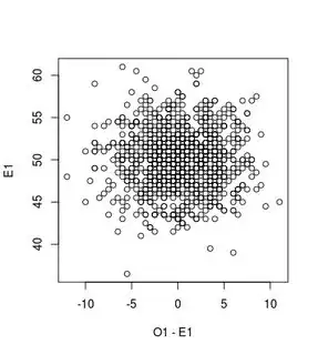
independence

set.seed(1)
O1 = rbinom(n,100,0.5)
O2 = rbinom(n,100,0.5)
E1 = 0.5*(O1+O2)
plot(O1-E1, E1)
Sextus Empiricus
  • 43,080
  • 1
  • 72
  • 161
  • Thank you, that is helpful. I wonder if your two points are sufficient by themselves, or is my point also needed to show that "this is not a problem" (w.r.t. the OP's question). My intuition was that my point was of first-order importance, but perhaps it is not? In other words, if the variance of the distribution of the difference between the true and the estimated $E_i$ did not shrink with the sample size and stayed as large as with $n=1$, would this be a problem? – Richard Hardy Jan 10 '22 at 07:10
  • I see mainly 2 points of which the 2nd relates to yours, but it is only in the denominator where it counts. So we have **1** The influence of $E_i$ is very small in the numerator term $E_i-O_i$ because of the (approximate) independence. This is independence is not because $E_i$ approaches a constant (law of large numbers) but instead because the observations approach a multivariate normal distribution (where the parameters like $O_1 - O_2$ and $O_1+ O_2$ are independent). **2** There is some influence of the parameter $E_i$ in the denominator. In that place you get that your point plays a role – Sextus Empiricus Jan 10 '22 at 07:15
  • You got deeper into the matter than I intended (and that is good). My original confusion concerned how presentations of $\chi^2$ test get away by saying $E_i$ is the expected value when it is actually only an estimate thereof, and then basing the intuition on how $O_i$ should not be far from the expected value under $H_0$. I remember being confused the first time I heard the argument, but I never got to think about it in any depth. When I remembered the issue 15 years later, it dawned on me that I now had some intuition as to why it works in spite of the discrepancy. (Why? Because it shrinks). – Richard Hardy Jan 10 '22 at 07:22
  • So my original concern did not go as far as to question whether $\frac{(\text{observed}_i-\text{expected}_i)^2}{\text{expected}_i}$ is actually $\chi^2$ distributed, it stopped earlier. In the meantime, your answer addresses a fuller point, I suppose. – Richard Hardy Jan 10 '22 at 07:26
  • @RichardHardy I remember that the first time that I came across the $\chi^2$ test I was wondering why it isn't (O-E)^2/O instead of (O-E)^2/E. It was only when I read Pearson's 1900 article that I came to view the $\chi^2$ test as an equivalent to a linear regression where we can have a geometrical view of [the distribution of the observations as a n-dimensional cloud that partitions into two spaces with dimensions n-p and p](https://stats.stackexchange.com/a/516882/164061). – Sextus Empiricus Jan 10 '22 at 07:45
0

No, it is generally not a problem. Consider the probability distribution of the difference between $E_i$ and the corresponding true value. The empirical $E_i$ converges to the corresponding true expected value fast enough (how fast: think Law of Large Numbers and Central Limit Theorem) so that the difference between the empirical and the true $E_i$ is asymptotically negligible compared with the difference between $O_i$ and $E_i$. Thus, the intuitive argument goes through despite $E_i$ being an estimate rather than the true value.

Richard Hardy
  • 54,375
  • 10
  • 95
  • 219
  • I added an answer that shows that there is more to it than just the $E_i$ converging to the true value. What we have in addition is that we can see this as $(E_i- O_i)^2$ as a variable that is independent of $E_i$. If $E_i$ is larger, then this is because $O_i$ (and some other values) are larger. The $E_i$ and $O_i$ are correlated. The result is that $(E_i- O_i)^2$ is nearly independent from $E_i$. – Sextus Empiricus Jan 09 '22 at 21:41