This is to complement rather than to disagree with @ChristianHenning's Answer and Comments.
It is the residuals of the t-test that need to be
normal. So if you have Sample 1 $X_1, X_2, \dots, X_n$
and Sample 2 $Y_1, Y_2, \dots Y_m,$ then you might
make a normal probability plot of the $m+n$ differences $$X_1 - \bar X, X_2, - \bar X, \dots, X_n - \bar X,\:\; Y_i - \bar Y, \dots Y_m-\bar Y.$$ However, your normal probability plot of the $Y_i$ is sufficiently non-normal (perhaps exponential?) to lead to a non-linear normal probability plot of residuals.
It may not be quite enough for $\bar X - \bar Y$ to be nearly normal. Only for normal data are the sample mean and sample variance stochastically independent. Thus, if data are not normal the t statistic (with information from the means in the numerator and information from
the variances in the denominator) may not have a t distribution, leading to a t test that is misleading.
If we use a nonparametric Wilcoxon Rank Sum test to compare two distributions of remarkably different shapes, and if we reject the null hypothesis, indicating that the
two samples have significantly different 'locations', then it may not be entirely clear what to conclude.
The correct conclusion may have to do with differences in location (medians) or indicate 'stochastic domination' of one sample over the other.
In particularly problematic cases, it may be helpful to do a permutation test of the null hypothesis that the two samples come from populations with the same mean and the alternative that population means differ.
Illustrating permutation tests. Whatever its distribution may be, you may feel that
a two-sample t statistic does a good job of reflecting differences in means. Then you can randomly permute
observations between the x and y samples and
find the value of the t statistic for each such permutation. With enough iterations of such permutations, one can get a good idea of the permutation distribution of the t statistic, and of the P-value of test of the null hypothesis against
the alternative.
For example, consider the following fictitious data
in which the two populations have normal and exponential distributions with the same mean.
set.seed(2021)
x = rnorm(20, 50, 10)  # mean 50
y = rexp(40, 1/50)     # mean 50
z = c(x,y)             # all 60 observations
g = rep(1:2, c(20,40))
pv.obs = t.test(z ~ g)$p.val  # obs p-val Welch
pv.obs
0.8331715
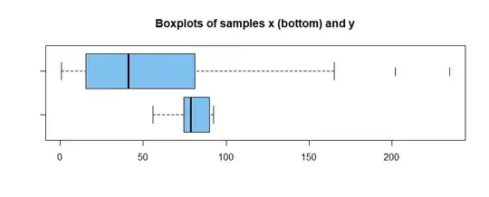
Boxplots illustrate different shapes of the two samples.
hdr = "Boxplots of samples x (bottom) and y"
boxplot(x, y, col="skyblue2", horizontal=T, pch="|",main=hdr)
[In this scenario a Wilcoxon rank sum test does not reject at the 5% level. R code wilcox.test(x, y)$p.val returns $0.105.]$
In the R code below for the permutation test, the
expression sample(g) makes the random assignments of all data among two samples of size2 20 and 40.
set.seed(1222)
pv.prm = replicate(10^5,
          t.test(z~sample(g))$p.val)
mean(pv.prm <= pv.obs)
[1] 0.83924           # aprx P-val of perm test
2*sd(pv.prm <= pv.obs)/sqrt(10^5)
[1] 0.00232308        # aprx 95% margin of sim error
Thus, the simulated P-value of the permutation
test is $0.839 \pm 0023,$ which exceeds 5%, so that
the null hypothesis is not rejected.
By contrast, if the fictitious data are from
populations of different shape with means $\mu_x = 75$ and $\mu_y = 50,$ then a permutation test rejects
the null hypothesis (P-value about $0.015 < 0.05 = 5\%)$ that population means are equal.
set.seed(2021)
x = rnorm(20, 75, 10)  # mean 75
y = rexp(40, 1/50)     # mean 50
z = c(x,y)             # all 60 observations
g = rep(1:2, c(20,40))
pv.obs = t.test(z ~ g)$p.val  # obs p-val Welch
pv.obs
[1] 0.0149717

hdr = "Boxplots of samples x (bottom) and y"
boxplot(x, y, col="skyblue2", horizontal=T, pch="|",main=hdr)
[In this scenario a Wilcoxon rank sum test rejects at the 5% level. R code wilcox.test(x, y)$p.val returns $0.015.$ The interpretation of 'rejection' may be controversial.]
set.seed(1222)
pv.prm = replicate(10^5,
           t.test(z~sample(g))$p.val)
mean(pv.prm <= pv.obs)
[1] 0.01476
In this example the P-value of the permutation test, using the Welch 2-sample t statistic as metric, gives about the same P-value as the Welch test. In both parts of this
example $(H_0$ true and not), $n=50$ observations from the exponential
distribution seems to be enough to rely on the legendary robustness of t tests against departures
from normality.
In reporting the results, we might just say that 50 is enough, and that we verified this via a permutation test. Alternatively, one we might say we were not
confident using the Welch t test with such skewed
data in Sample 2, so we did a permutation test, and
report results of the permutation test.


