A Frequentist approach to modeling uncertainty around decision optimization

Question

I'm curious about how a Frequentist would approach an optimization problem, where said problem is constructed using inferred parameters. As an example, I'll use price optimization given a demand curve. $Revenue(x) = Price * Volume$. Let's assume my demand curve follows exponential decay.

1. Infer demand curve parameters
2. Maximize $Revenue(X)$

I can perform linear regression, given price and the log of the sales volume, to infer the slope and intercept. Using a Bayesian approach, I'll have a posterior chain to sample from. So, if I have 4000 samples in my posterior chain, I can uniformly draw indices in the range [1, 4000], and retrieve their corresponding slope and intercept values then use them to visualize my revenue function.

Big edit: Code included

• simulate data

sd = 0.5
m,b = -0.25, 5
X = np.linspace(0,20,100)
Y = np.exp(np.random.normal(loc=m*X+b, scale=sd))
plt.scatter(X,Y)

• Model w/ PyMC3

with pm.Model() as model:
  m = pm.Normal('m',mu=0, sd=2)
  b = pm.Normal('b',mu=0, sd=2)
  s = pm.Exponential('s',lam=1)
  y_hat = pm.math.dot(m, X) + b
  lik = pm.Normal('lik', mu=y_hat, observed=pm.math.log(Y), sigma=s)
  trace = pm.sample(chains=4)

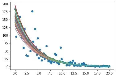
• plot posterior-predictive distribution

def post_plot(trace_obj=trace,samples=100,size=len(X)):
  for itr in range(samples):
    idx = random.choice(range(size))
    m = trace_obj.get_values('m')[idx]
    b = trace_obj.get_values('b')[idx]
    Y_hat = np.exp(m*X + b)
    plt.plot(X,Y_hat)
  plt.scatter(X,Y)

post_plot()  

• Posterior predictive revenue

def rev_posterior(samples=100, size=len(X)):
  for s in range(samples):
    idx = random.choice(range(size))
    m = trace.get_values('m')[idx]
    b = trace.get_values('b')[idx]
    rev = X * np.exp(m*X +b)
    plt.plot(X, rev)
  return 

rev_posterior()  

.

This is useful in two ways: (A) I can see the variance around the sales volume at the optimal price. And (B) I can see that each sampled function has a peak around the same spot; in other words, there's very little variance around where the optimal price is located.

My actual question: Using parameter estimates and confidence intervals, how might a Frequentist construct a similar revenue function plot? I understand that they could simply use the point estimates of the slope and intercept and then find a point estimate of the optimal price, but I'm curious about the variance around the optimal value.

For the code that simulated this data, generated this plot, and Bayesian model that inferred the posterior distribution, see here

Answer 1

For uncertainty concerning an unknown fixed true parameter the frequentist would construct a confidence interval. This can be viewed as the inversion of a hypothesis test to identify the set of plausible values for a parameter given the observed data.

The frequentist can use these parameter estimates (slope and intercept) to estimate the unknown fixed true mean revenue and construct a confidence band. This is also based on the inversion of a hypothesis test. Most of the time it is a Wald or t-test that is inverted to form a confidence interval. When dealing with non-normal data a proper link function (transformation of the parameter and the estimator) will yield an estimator that approximately follows a normal distribution. The Wald test can be safely inverted for the transformed parameter, and the confidence limits back-transformed to the scale of interest. Think of logistic regression where the estimator for the log odds is well-approximated by a normal distribution. By using the inverse link function we can obtain confidence limits for the population proportion. Let me know if you need more details. This link function approach is also used in Bayesian inference so that a normal distribution can be used for the prior and posterior.

Here is an answer providing a couple of ways to construct a confidence interval for a binomial proportion and to visualize this inference using a confidence curve, analogous to a Bayesian posterior. Here is a discussion of hypothesis tests and confidence intervals, and how they are all approximations to the likelihood ratio test.