If the correlation between $Y \alpha $ and $X \beta$ is maximized then the $\beta$ are such that it is the OLS solution of $\alpha Y$ (where we either translate the columns in $X$ such that the column means are zero, or we add an intercept to the OLS regression).
So we have $$X \beta = X(X^T X)^{-1}X^TY \alpha = Y_{\parallel} \alpha$$
the difference is
$$X \beta - Y \alpha = (X(X^T X)^{-1}X^T-I)Y \alpha = Y_{\perp} \alpha$$
The image below illustrates this in 3 dimensions.
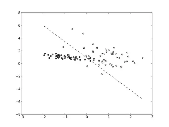
The possible solutions $Y\alpha$ and $X\beta$ are in a surface spanned by the vectors $Y_1, Y_2, ... Y_n$ and $X_1, X_2, ... X_n$. For a given $\alpha$ the solution of $\beta$ that minimizes the correlation is the OLS solution, ie. the perpendicular projection of $Y\alpha$ onto the surface spanned by $X$.
In this example with 3D coordinates we see that the planes intersect and $\alpha$ can be changed such that the vector $Y\alpha$ is entirely in the plane spanned by $X$. And the correlation can be made equal to 1. But in more dimensions, the hyper-surfaces might not need to intersect (except in the point zero where the planes always intersect).
Solution with optimization using a Lagrangian function
Maximizing the correlation between $X \beta $ and $Y \alpha$ is like minimizing the ratio of the length of the vectors $Y_{\perp} \alpha$ and $Y_{\parallel} \alpha$ or $Y \alpha$. The correlation is larger for a smaller remainder $Y_{\perp} \alpha$ while keeping the projection $Y_{\parallel}\alpha$ or total vector $Y \alpha$ the same size.
We can solve this by minimizing the Lagrangian
$$L(\alpha, \lambda) = \alpha^T \, M_{\perp} \, \alpha + \lambda(\alpha^T \, M \, \alpha - 1)$$
where $M_{\perp} = Y_{\perp}^TY_{\perp}$ and $M = Y^TY$
whose gradient must be zero leading to the equations
$$ \begin{array}{}
(M_{\perp}+\lambda M) \alpha &=& 0 \\
\alpha^T\,M \, \alpha &=& 1
\end{array}$$
To solve the first equation, we are looking for a constant $\lambda$ and vector $\alpha$ such that
$$M_{\perp}\alpha = -\lambda M \alpha $$
or
$$(M^{-1}M_{\perp}) \alpha = -\lambda \alpha $$
Which makes the $-\lambda$ and $\alpha$ the eigenvalues and eigenvectors of $(M^{-1}M_{\perp})$.
The solution with the maximum correlation will be related with the smallest eigenvalue $\lambda_v = -\lambda$. This is because we can compute the correlation as
$$\rho = \sqrt{1-\frac{\alpha^T \, M_{\perp} \, \alpha }{\alpha^T \, M \, \alpha }} = \sqrt{1-\frac{\alpha^T \, \lambda_v M \, \alpha }{\alpha^T \, M \, \alpha }} = \sqrt{1-\lambda_v} $$
So an algorithm to find $\alpha$ and $\beta$ is to compute the eigenvectors of that matrix and select the one with the smallest absolute value of the eigenvalue.
Code example
library(MASS)
set.seed(1)
### create X and Y
X = t(mvrnorm(3,mu = rep(0,10), Sigma = diag(10) ))
Y = t(mvrnorm(3,mu = rep(0,10), Sigma = diag(10) ))

### subtract the means (without loss of generality)
X = X - rep(1,10) %*% t(colMeans(X))
Y = Y - rep(1,10) %*% t(colMeans(Y))

### compute matrices
P = X %*% solve(t(X) %*% X) %*% t(X)  ### projection matrix
Ypar = P %*% Y                        ### Y projected on X
Yperp = Y-Ypar                        ### residual of projection
M = t(Y) %*% Y               ### quadratic form to compute square length
Mperp = t(Yperp) %*% Yperp


### solve with eigenvectors
eV = eigen(solve(t(M)) %*% Mperp)$vectors


### compute Xbeta and Yalpha
### when putting alpha equal to the last eigenvector
### the last eigenvalue is the one with the lowest eigenvalue
alpha = alpha = eV[,length(eV[1,])]
yfit = Y %*% alpha
xfit = P %*% yfit
corrV = cor(yfit,xfit)


### optimization of correlation
f<-function(p){
  a1 = p[1:3]
  a2 = p[4:6]
  rho = cor((Y %*% a1),(X  %*% a2))
  d = abs(sum(a1^2)-1)^2
  return(-rho+d)
}

a = rep(1,6)
### optimize correlation
mod <- optim(a,f, method = "BFGS",control = list(maxit=1*10^5,trace=1,reltol=10^-16))
mod

### check results of models
yh = Y %*% mod$par[1:3]
xh = X %*% mod$par[4:6]

### correlation from optimization
### 0.69886626
cor(yh,xh)

### correlation from eigenvectors
### 0.6988626 (it's the same)
max(corrV)
Intuition
The correlation in terms of the vector $\alpha$ is the ratio of the length of the vectors
$$\rho = \frac{\Vert Y_{\parallel} \alpha \Vert}{\Vert Y \alpha \Vert} = \sqrt{\frac{\alpha^T \, M_{\parallel} \, \alpha}{\alpha^T \, M \, \alpha}} =\sqrt{\frac{\alpha^T \, M^{-1} M_{\parallel} \alpha}{\alpha^T\alpha}}$$
If we restrict the $\alpha$ to be of a specific size then the alpha that maximizes this product $\alpha^T \, M^{-1} M_{\parallel} \, \alpha$ is directed along the eigenvector with the largest eigenvalue.
